Forest plot for meta-analysis displaying the mean ES with and without outliers

Question

I am conducting a meta-analysis and am trying to produce a forest plot displaying the mean weighted effect size with and without the outliers. I looked on so many websites and tried a lot of syntaxes, however, didn't really find anything about what I am looking for.

Assume there are 10 studies in the meta-analysis. Outlier analyses showed that Study 3 is an outlier leading to an overestimation of the mean weighted ES. Accordingly, I calculate a mean ES with (k = 10) and without the outlier (k = 9). I would like to display the studies sorted according to their ES and report both Mean ESs in the forest plot. I would appreciate any help and/or advice.

Study3 Study9 Study5 ... Study7

Mean ES (k = 10) Mean ES (k = 9)

---

Thank you again for your response. I have been able to produce the graphs I wanted, there were only two issues, and I was wondering if there is an easier way to do it than I did.

APA style requires to write statistical terms italic, e.g., k = 10, and at sometimes also subscripted, e.g., u in Hedges g[u]. My apologies, the subscript command here seems not to work. I tried this syntax to finish the forest plot but without success as the program would draw the ** and [], as well as the command "italic()" in the graphs.

Further, the command digits=2 was successful for the single ES and CIs, however not for the tables left hand side where I have mean age and the mean scores for each of the experimental groups (Note: the DV is continuous).

I created a syntax as follows, however, as I said, I was wondering if there is an easier was to do this. The meta-analyses for each of the subgroups have been already calculated.

### decrease margins so the full space is used
par(mar=c(4,4,1,2))

### draw a plot
par(font=1)
with(SMetaHits, forest(rma.allHits, xlim=c(-12,  6), ylim=c(-1, 41),
                       xlab="Hedges gu", slab=paste(author), 
                       ilab=cbind(SMetaHits$N, SMetaHits$MYou, SMetaHits$MOld), 
                       ilab.xpos=c(-6, -4.5, -3.5), ilab.pos=c(2, 4, 4),
                       order=order(SMetaHits$FacAgeNum), rows=c(36:30, 24:15, 9:4)))
text(-12, 40, "Author(s), Year [Exp.]", pos=4)

### add text for the subgroups
par(font=3)
text(-12.1, c(37.5,25.5,10.5), pos=4, c("Young", "Mixed-age", "Old"))

This is where it gets complicated and I was hoping that there is an easier way than this

### add column headings to the plot and draw Y and O subscripted and italic
par(font=3)
text(c(-6), 40, c("N"), pos=2)
text(c(-4.5, -3.5), 40, c("M", "M"), pos=4)
text(c(-4.3, -3.3), 39.7, c("Y", "O"), pos=4, cex=.75) ##Y and O subscripted

###Command to draw 0 to the mean scores; otherwise e.g., .6 instead of .60. 
par(font=1)
text(-3.75, c(36,16,4), "0", pos=2) ###add 0 to MY 
text(-2.75, c(7,4), "0", pos=2) ###add 0 to MO

At this stage, there were 2 problems: 1. I chose pos=2 to have all values left handed, which is a good solution only if the values are all in the same direction. As soon as there is one value negative, the values are not exactly underneath each other anymore. There are a lot of trial and errors to get the 0 at the right place, a similar problem I had below with gu

###Command to write Hedges *gu* as required, i.e., gu italic and u subscript. 
text(6, 40, "Hedges     [95% CI]", pos=2)  
par(font=3)  
text(4.93, 40, "g", pos=2)
text(5.02, 39.7, "u", pos=2, cex=.75)

The last command, I noticed only now that k is not italic yet

### add summary polygons for the three subgroups 
par(font=2)
addpoly(res.YoF, row=28.5, cex=1, mlab="FE Model (k = 7)")
addpoly(res.YoFNoOutl, row=27.3, cex=1, mlab="FE Model (k = 6)")
addpoly(res.MxF, row=13.5, cex=1, mlab="FE Model (k = 10)")
addpoly(res.MxFNoOutl, row=12.3, cex=1, mlab="FE Model (k = 9)")
addpoly(res.OlF, row=2.5, cex=1, mlab="FE Model (k = 6)")
addpoly(res.OlFNoOutl, row=1.3, cex=1, mlab="FE Model (k = 5)")}'

Answer 1

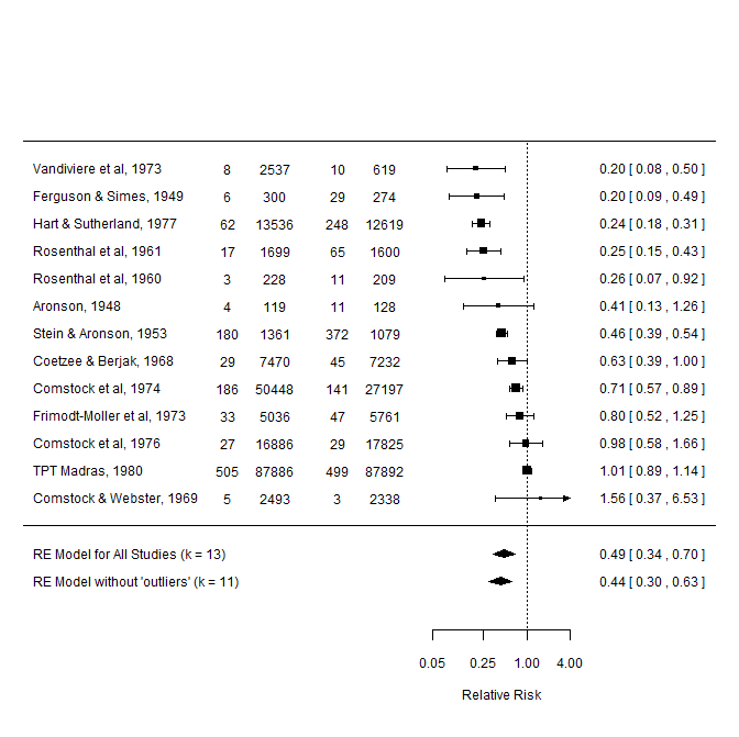
You missed metafor's function addpoly(). Here is a fully reproducible example:

library(metafor)

data(dat.bcg)

## REM (k = 13)
res <- rma(ai=tpos, bi=tneg, ci=cpos, di=cneg, data=dat.bcg, measure="RR",
           slab=paste(author, year, sep=", "), method="REML")

## REM (k = 11; 'outliers' removed)
res2 <- rma(ai=tpos, bi=tneg, ci=cpos, di=cneg, data=subset(dat.bcg, trial < 12),
            measure="RR", slab=paste(author, year, sep=", "), method="REML")

## Forest plot
forest(res, xlim=c(-16, 6), at=log(c(.05, .25, 1, 4)), atransf=exp,
       ilab=cbind(dat.bcg$tpos, dat.bcg$tneg, dat.bcg$cpos, dat.bcg$cneg),
       ilab.xpos=c(-9.5,-8,-6,-4.5), cex=.75, ylim=c(-3, 16),
       order="obs", xlab="Relative Risk", mlab="RE Model for All Studies (k = 13)")

## Add second summary effect size
addpoly(res2, atransf=exp, mlab="RE Model without 'outliers' (k = 11)", cex=.75)

Here is the result:

Update:

• Use expression() to include subscripts etc.: xlab = expression("Hedges " * g[u]).
• Use italic() within expression to get italic statistical terms: expression(italic("Hedges " * g[u]))
• The proper alignment of the table seems tricky, I doubt there is a simple solution avaliable...

Here is an update of the R code and the plot:

library(metafor)

data(dat.bcg)

## REM (k = 13)
res <- rma(ai=tpos, bi=tneg, ci=cpos, di=cneg, data=dat.bcg, measure="RR",
           slab=paste(author, year, sep=", "), method="REML")

## REM (k = 11; 'outliers' removed)
res2 <- rma(ai=tpos, bi=tneg, ci=cpos, di=cneg, data=subset(dat.bcg, trial < 12),
            measure="RR", slab=paste(author, year, sep=", "), method="REML")

## Forest plot
forest(res, xlim=c(-16, 6), at=log(c(.05, .25, 1, 4)), atransf=exp,
       ilab=cbind(dat.bcg$tpos, dat.bcg$tneg, dat.bcg$cpos, dat.bcg$cneg),
       ilab.xpos=c(-9.5,-8,-6,-4.5), cex=.75, ylim=c(-3, 16),
       order="obs",xlab = expression(italic("Hedges " * g[u])), mlab="RE Model for All Studies (k = 13)")

## Add second summary effect size
addpoly(res2, atransf=exp, mlab="RE Model without 'outliers' (k = 11)", cex=.75)