The standard deviation is as applicable here as anywhere else: it gives useful information about the dispersion of the data. In particular, the sd divided by the square root of the sample size is one standard error: it estimates the dispersion of the sampling distribution of the mean. Let's calculate:
$$3.2\% / \sqrt{10000} = 0.032\% = 0.00032.$$
That's tiny--far smaller than the $\pm 0.50\%$ precision you seek.
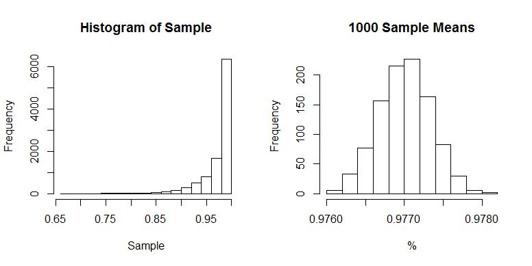
Although the data are not Normally distributed, the sample mean is extremely close to Normally distributed because the sample size is so large. Here, for instance, is a histogram of a sample with the same characteristics as yours and, at its right, the histogram of the means of a thousand additional samples from the same population.

It looks very close to Normal, doesn't it?
Thus, although it appears you are bootstrapping correctly, bootstrapping is not needed: a symmetric $100 - \alpha\%$ confidence interval for the mean is obtained, as usual, by multiplying the standard error by an appropriate percentile of the standard Normal distribution (to wit, $Z_{1-\alpha/200}$) and moving that distance to either side of the mean. In your case, $Z_{1-\alpha/200} = 2.5758$, so the $99\%$ confidence interval is
$$\left(0.977 - 2.5758(0.032) / \sqrt{10000},\ 0.977 + 2.5758(0.032) / \sqrt{10000}\right) \\ = \left(97.62\%, 97.78\%\right).$$
A sufficient sample size can be found by inverting this relationship to solve for the sample size. Here it tells us that you need a sample size around
$$(3.2\% / (0.5\% / Z_{1-\alpha/200}))^2 \approx 272.$$
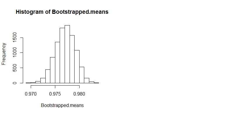
This is small enough that we might want to re-check the conclusion that the sampling distribution of the mean is Normal. I drew a sample of $272$ from my population and bootstrapped its mean (for $9999$ iterations):

Sure enough, it looks Normal. In fact, the bootstrapped confidence interval of $(97.16\%, 98.21\%)$ is almost identical to the Normal-theory CI of $(97.19\%, 98.24\%)$.
As these examples show, the absolute sample size determines the accuracy of estimates rather than the proportion of the population size. (An extreme but intuitive example is that a single drop of seawater can provide an accurate estimate of the concentration of salt in the ocean, even though that drop is such a tiny fraction of all the seawater.) For your stated purposes, obtaining a sample of $10000$ (which requires more than $36$ times as much work as a sample of $272$) is overkill.
R code to perform these analyses and plot these graphics follows. It samples from a population having a Beta distribution with a mean of $0.977$ and SD of $0.032$.
set.seed(17)
#
# Study a sample of 10,000.
#
Sample <- rbeta(10^4, 20.4626, 0.4817)
hist(Sample)
hist(replicate(10^3, mean(rbeta(10^4, 20.4626, 0.4817))),xlab="%",main="1000 Sample Means")
#
# Analyze a sample designed to achieve a CI of width 1%.
#
(n.sample <- ceiling((0.032 / (0.005 / qnorm(1-0.005)))^2))
Sample <- rbeta(n.sample, 20.4626, 0.4817)
cat(round(mean(Sample), 3), round(sd(Sample), 3)) # Sample statistics
se.mean <- sd(Sample) / sqrt(length(Sample))      # Standard error of the mean
cat("CL: ", round(mean(Sample) + qnorm(0.005)*c(1,-1)*se.mean, 5)) # Normal CI
#
# Compare the bootstrapped CI of this sample.
#
Bootstrapped.means <- replicate(9999, mean(sample(Sample, length(Sample), replace=TRUE)))
hist(Bootstrapped.means)
cat("Bootstrap CL:", round(quantile(Bootstrapped.means, c(0.005, 1-0.005)), 5))


