How exactly does null hypothesis testing work

Question

I'm trying to gain a better understanding of how null hypothesis testing works.

I have 3 questions related to the code below:

1. Am I right in saying the probability of each t value in t_distribution should follow the tables of critical values for t distributions found in statistical text books?

2. If yes, how using R code, can I show t_distribution follows the tables of critical values for t distributions found in statistical text books

3. Who exactly made the tables of critical values for t distributions found in statistical text books?

make 2 populations with (almost) zero difference

population1 <- rnorm(10000, 3, 2)
population2 <- rnorm(10000, 3, 2)

sample 100 values from each population

library(plyr)
population1_5000_samples <- llply(1:5000, function(x) sample(population1, 100, replace = F))
population2_5000_samples <- llply(1:5000, function(x) sample(population2, 100, replace = F))

do 5000 t-tests and extract t values

t_distribution <- laply(1:5000, function(x) t.test(population1_5000_samples[[x]], population2_5000_samples[[x]])$stat)

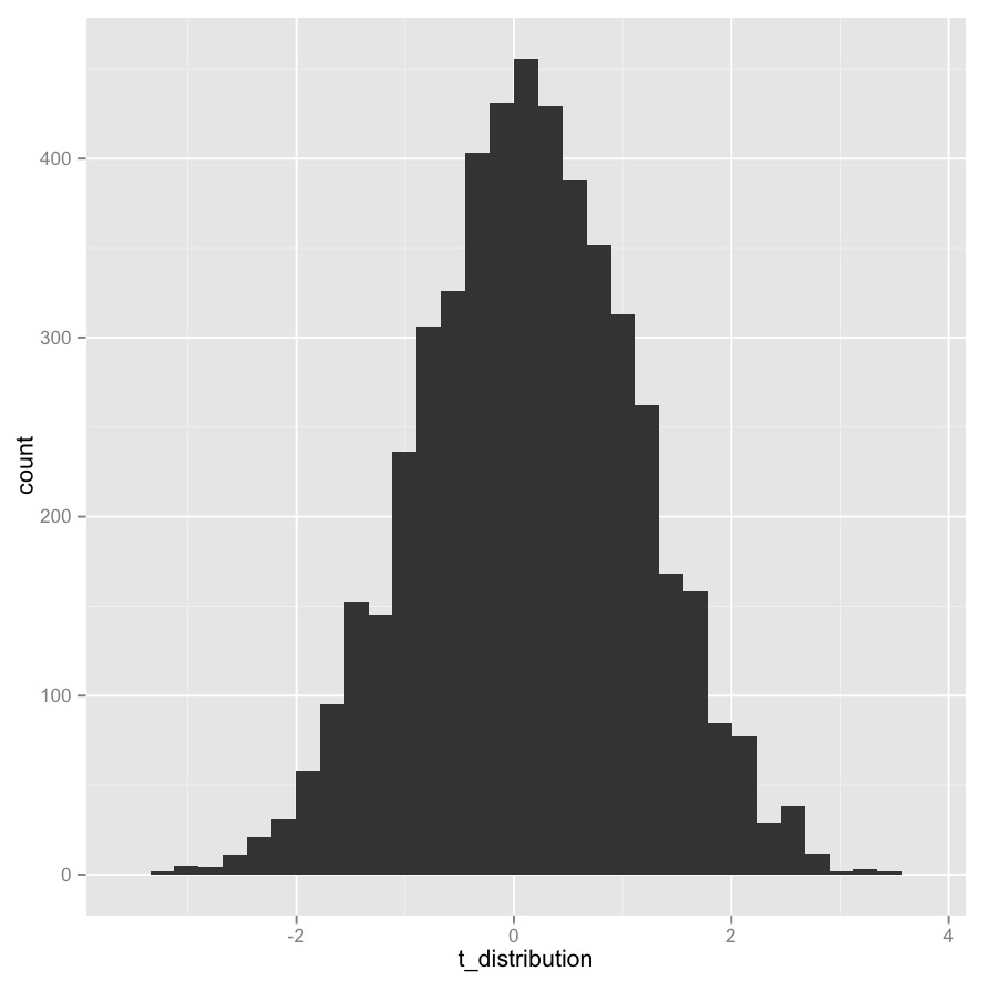
distribution of t values

library(ggplot2)
ggplot(as.data.frame(t_distribution), aes(t_distribution)) + geom_histogram()

Answer 1

Actually, your code will not generate values from a t-distribution (not quite, at least).

This is because t.test by default uses the Welch test.

There are two things that prevent your results having a t-distribution:

i) the Welch-statistic only has approximately a t-distribution -- the denominator is only approximately chi-square with the nominal df of the Welch test.

ii) the df are computed as a function the sample values, and thus vary each time you generate a new sample. Thus you'll actually get some mixture of these not-quite-t-distributions-that-are-conditional-on-sample-specific-variance-ratios.

---

Here's how to actually get a t-distribution; if you want a two-sample t-test, you'll need to use an equal-variance t-test:

n <- 10 # this will get you a t with 18 df
res <- replicate(5000,{x=rnorm(n);y=rnorm(n);(mean(x)-mean(y))/sqrt((var(x)+var(y))/n)})

This statistic is a simplified version (because of equal sample size) of an ordinary equal variance two-sample t-statistic.

Alternatively, if you want to use t.test:

n <- 10 # this will get you a t with 18 df
res <- replicate(5000,t.test(rnorm(n),rnorm(n),var.equal=TRUE)$statistic)

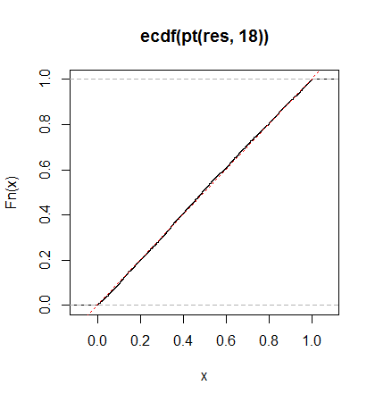
You can check it gives a t-distribution with the supposed d.f. by transforming the output using the cdf and comparing the result with a uniform:

plot(ecdf(pt(res,2*n-2)))
abline(0,1,col=2,lty=3)

giving

However, it's probably simpler to start with a one-sample test.

---

Who exactly made the tables of critical values for t distributions found in statistical text books?

Each set of tables - unless it credits someone else as a source - will likely have been constructed from scratch, in a variety of ways depending on when they were published.

Critical values are effectively tables of the inverse cdf, but if you can compute the cdf you can find the value that corresponds to a certain point of the cdf relatively quickly (e.g. via interpolation and say a Newton or secant-method step); there were also approaches like the use of finite difference methods that could also be used to achieve smooth interpolated results in use before people used computers for everything.

Note that for moderate to low d.f. it's quite reasonable to compute integrals directly (you can use integration by parts to write it in terms of an integral with d.f. that is two lower than the original, and the two lowest d.f. yield to standard integration methods. There's also numerical integration, which can be made quite accurate. There are series approximations, and there are highly accurate functional approximations (if I recall correctly, some are found in Abramowitz and Stegun for example). There are particular (highly accurate) functional approximations that are suitable for computer implementation, which is how tables are constructed now.

A typical set of t-tables might contain 100 to 200 values to about 3 or 4 figure accuracy; these could be computed by hand in a fairly short period of time - probably a couple of days at most if you have several people checking the computations (people who did such computations - often on mechanical calculators - were called computers). Perhaps 3 or 4 days with a single person doing the calculations and the checking.

The t-distribution itself dates back a long way; to Helmert in the mid 1870s (who was also responsible for the chi-square). Its use for the t-test is due to Gosset ("Student"), but I think the first tables of the inverse cdf for that purpose would be due to Fisher. For example, he gave t-tables in his 1925 book Statistical Methods for Research Workers (see the bottom of the page).

However, as mentioned by Fisher here (1922)$^{[1]}$, Gosset produced tables of the probability integral (i.e. the cdf rather than the inverse cdf) in 1917$^{[2]}$ (up to 30df); it would be practically possible to do the t-test from those. Indeed, Gosset's 1908 paper $^{[3]}$ has* a table for an integral related to the cdf of the $t$ for a set of small d.f. from which (with a little additional work), it's actually possible to in effect do t-tests (as he does in the paper, though keep in mind the hypothesis testing framework we're used to isn't entirely in place at that time).

*(see p19 here; a link to a scan of the original paper is on the Wikipedia page for the Student's t distribution, see note 9)

---

[1] Fisher, R.A. (1922),
"The goodness of fit of regression formulae, and the distribution of regression coefficients".
Journal of the Royal Statistical Society 85 (4): 597–612.

[2] Student, (1917),
"Tables for estimating the Probability that the Mean of a unique Sample of Observations lies between $-\infty$ and any given Distance of the Mean of the Population from which the Sample is drawn",
Biometrika 11 (4): 414-417

[3] Student, (1908),
"The probable error of a mean",
Biometrika 6 (1): 1–25.

Answer 2

To answer your last question, note that a random variable $T$ defined as such (letting $X\sim N(0,1)$ and $V\sim \chi_{n}^{2}$)

$$T=\frac{X}{\sqrt{V/n}}$$

If $Z$ and $V$ are independent then we say $T$ has a $t$-distribution with $n$ degrees of freedom. Now notice for a critical value $t^{*}$, that the table tells you $Pr(T\leq t^{*})$. Well in order to find this value you can integrate over the pdf of $T$. Since it is well known what pdfs of standard normal and chi square with degrees of freedom $n$ (which is just $\text{Gamma}(\frac{n}{2},\frac{1}{2}$)) there are methods to derive the pdf of $T$ which gives us this formula for the pdf

$$f_{T}(x)=\frac{\Gamma(\frac{n+1}{2})}{\sqrt{n\pi}\Gamma(\frac{n}{2})}\left(1+\frac{x^{2}}{n}\right)^{-\frac{n+1}{2}}\,.$$

Thus all the table is doing is for given $t^{*}$, it's calculating

$$Pr(T\leq t^{*})=\int^{t^{*}}_{-\infty}\frac{\Gamma(\frac{n+1}{2})}{\sqrt{n\pi}\Gamma(\frac{n}{2})}\left(1+\frac{x^{2}}{n}\right)^{-\frac{n+1}{2}}dx$$

which turns out can't be calculated explicitly so they designed a table that calculates this integral using numerical approximation techniques. So techically, as long as you know how to perform these numerical approximation techniques with integrals you could make a table yourself

Also if you want to show simulations from a $t$ distribution follow a distribution. as good check is to plot the density of the $t$ distribution given by table over histogram with following code

lines(density(qt(seq(0,1,by=0.05),df=n))

the qt and pt functions should give values that would be given in a book.

Now if you want to see if there is statistically significant that your simulation fits a $t$ distribution (i.e. perform hypothesis test) then you would want to perform the Kolmogorov-Smirnov test.

Answer 3

If I understand correctly, your question revolves around whether or not the t-values presented in statistical textbooks are generated by simulation. Generally these values are calculated (with the assistance of software) from the probability density function of the t-distribution. You can verify the accuracy of the tables in a textbook using the R function qt(). For example,

qt(.95,10)

returns the value 1.812461 which agrees with the statistical tables in Howell's Fundamental Statistics for the Behavioral Sciences (1.812) for a one-tailed test at alpha of .05 with 10 degrees of freedom. The source of the table in that book is listed as author calculation.

Run

?qt()

in R for more information.

Answer 4

The answer to your first question is yes, the t-values should be equivalent within a certain margin of error. They're calculated using a complicated mathematical formula that is the same regardless of whoever calculates values from it. R will almost certainly include more decimal places that your textbook author excluded due to space-related reasons. Imagine how big the table would be if every t-value had 6 or 7 decimal places!

Using R code, you could always generate a new table in a way similar to how Marcus described. You would get the same t-values but R would give you more decimal places.

The answer to your third question is a bit more complicated. Today it would almost certainly be done using software, but I wouldn't know how your textbook does it unless I knew the title. If you're wondering about the very first statistical tables, they probably would have been calculated using either variations of Newton's Method or interpolation. I can't seem to find any for the t-distribution at the moment, but Abramowitz and Stegun, a well-respected reference book from the 1950s, has a page on how to approximate values from a normal distribution. As you can see, it's really tricky!