1
$\begingroup$

I have repeated samples of geocoordinates of activities in a city. In most of these samples positions will simply be random. In some samples, however, some percentage of the data will be arranged -- with some error -- on a line. Let me paint you a picture (code to generate this data below):
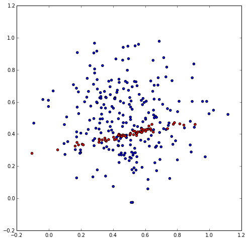
Scatter with line

I want to be able to

  • detect whether or not the sample contains a line
  • estimate the two parameters of this line from the data if it does

I've toyed with doing this with a Hough transform (see my previous question) but am struggling to make that work in a robust way. I have therefore tried to take another stab at the problem using a Bayesian mixture model. The code below generates model data and implements such a mixture model in PyMC, which works surprisingly well (note: most of my data will have p=0, the rest will have strictly positive p, anywhere from 0.2 to 0.5 I would guess):

import numpy as np
from matplotlib import pyplot as plt
import pymc as pm
import scipy.stats as stats

# DGP parameters
N = 300
p0 = 0.2
alpha0 = 0.3
beta0 = 0.2
sigma0 = 0.01
sigma_noise = 0.2

# DGP
x = np.random.normal(0.5,0.2,N)
y_line = np.random.normal(alpha0+beta0*x,sigma0)
line_bool = np.array(stats.bernoulli.rvs(p0, size=N))
y_rand = np.random.normal(0.5,0.2,N)
y_all = y_line*line_bool + y_rand*(1-line_bool)

# plot
fig = plt.figure(figsize=(8,8))
ax1 = fig.add_subplot(111,aspect='equal')
ax1.scatter(x[line_bool==0], y_all[line_bool==0],c='b')
ax1.scatter(x[line_bool==1], y_all[line_bool==1],c='r')

# prior for the assignment probability is a beta distribution that puts a lot of probability mass near 0
p = pm.Beta("p", 1, 3, value=0.5)
assignment = pm.Bernoulli("assignment", p, size=N)

# priors for the noise component
center_noise = pm.Normal("center_noise", 0.5, 0.4)
tau_noise = 1.0 / pm.Uniform("tau_noise", 0, 1) ** 2

# priors for the line parameters
beta_min = -10**1
beta_max = 10**1
line_pars = pm.Uniform("line_pars", beta_min, beta_max, size=2)
tau_line = 1.0 / pm.Uniform("tau_line", 0, 0.05) ** 2

# deterministic functions for the means and variances conditional on assignment
@pm.deterministic
def center_i(assignment=assignment, center_noise=center_noise, x=x, line_pars=line_pars):
    center_line = line_pars[0]+line_pars[1]*x
    return assignment*center_line + (1-assignment)*center_noise

@pm.deterministic
def tau_i(assignment=assignment, tau_noise=tau_noise, tau_line=tau_line):
    return assignment*tau_line + (1-assignment)*tau_noise

# define the observed variables
x_obs = pm.Normal("x_obs", 0.5, 0.2, value=x, observed=True)
y_obs = pm.Normal("y_obs", center_i, tau_i, value=y_all, observed=True)

# define the model
model = pm.Model([p, assignment, center_noise, tau_noise, line_pars, tau_line])

# sample from the posterior
mcmc = pm.MCMC(model)
map_ = pm.MAP( model )
map_.fit()
mcmc.sample(50000, 20000, 3)

# look at the posterior
from pymc.Matplot import plot as mcplot
mcplot(mcmc.trace("p", 2), common_scale=False)
mcplot(mcmc.trace("line_pars", 2), common_scale=False)
mcplot(mcmc.trace("tau_noise", 2), common_scale=False)
mcplot(mcmc.trace("tau_line", 2), common_scale=False)

This works well on generated data (though I would welcome suggestions for how to improve it!), but I suspect the real data this will have to work on will be a bit messier. In particular the "background noise" (y_rand above) isn't nicely normal. I'm therefore wondering how I would generalize the model above:

  • How would I define mixture models in which the mixture concerns not only the parameters of the distribution but the type of distribution (say, the background noise being uniformly distributed)?
  • How might I make the distribution of the background noise far more general. My data being geocoordinates of activities in a city, is there way a way of taking into account that even in the course of normal activity (with p=0) positions may more often be arranged along a line than the simple normal model above would suggest (e.g. because they take place along a straight road)? Is there a way of "diffing out" the kind of activity that usually takes place on a Wednesday afternoon when estimating the model on data from a new Wednesday afternoon?
$\endgroup$
7
  • $\begingroup$ You might be struggling with the Hough transform because the code in an answer to your previous question is incorrect. Using angular coordinates for the slopes and applying some straightforward image-processing filters tends to work pretty well. $\endgroup$
    – whuber
    Commented Aug 18, 2014 at 14:34
  • $\begingroup$ I believe the answer to my earlier question just gave the slope/intercept form of the Hough transform for reasons of simplicity. I've since coded this up using polar coordinates but that changes very little. My main problem is that I often get the line wrong if it existsand have no good way of determining whether or not there even is a line at all. What are the image-processing filters you would suggest? $\endgroup$
    – RoyalTS
    Commented Aug 18, 2014 at 15:41
  • $\begingroup$ The image processing is described in detail in my answer at stats.stackexchange.com/questions/33078. It comprises contrast enhancement, smoothing ("blurring"), and thresholding. My answer there applies directly to your example here and provides a working solution. It does not address your questions about parameter estimation or controlling for covariates such as seasonal indicators ("Wednesday afternoons," for instance). In your example you should be able to identify a large number of linear configurations of points. $\endgroup$
    – whuber
    Commented Aug 18, 2014 at 16:13
  • $\begingroup$ Interesting. You wouldn't, by any chance, still have the code you used to generate the answer to that question? $\endgroup$
    – RoyalTS
    Commented Aug 18, 2014 at 16:35
  • $\begingroup$ I actually do, so I inserted the relevant portions into my other answer. $\endgroup$
    – whuber
    Commented Aug 18, 2014 at 17:17

1 Answer 1

5
$\begingroup$

That's an interesting problem. I think it nicely highlights the power of Bayesian statistics as you can build these custom models based on how you think your data was generated and then invert them.

To answer your question: I would suggest to instead do the mixture inside of the likelihood where you can choose the specific likelihood function for each mixture component.

I rewrote your model a bit (and had to change some parameters and priors to make it work). You might need to adapt it to fit your bill but it should demonstrate the trick with the custom likelihood function I alluded to.

import numpy as np
from matplotlib import pyplot as plt
import pymc as pm
import scipy.stats as stats

# DGP parameters
N = 300
p0 = 0.5
alpha0 = 0.3
beta0 = 0.2
sigma0 = 0.01
sigma_noise = 1.0

# DGP
x = np.random.normal(0.5, 0.2, N)
y_line = np.random.normal(alpha0+beta0*x,sigma0)
line_bool = np.array(stats.bernoulli.rvs(p0, size=N))
y_rand = np.random.normal(0.5,0.2, N)
y_all = y_line*line_bool + y_rand*(1-line_bool)

# plot
fig = plt.figure(figsize=(8,8))
ax1 = fig.add_subplot(111,aspect='equal')
ax1.scatter(x[line_bool==0], y_all[line_bool==0],c='b')
ax1.scatter(x[line_bool==1], y_all[line_bool==1],c='r')

# prior for the assignment probability is a beta distribution that puts a lot of probability mass near 0.5
p = pm.Beta("p", 1, 10, value=0.5)
assignment = pm.Bernoulli("assignment", p, size=N)

# priors for the line parameters
intercept_prior = pm.Normal('intercept', 0, 10**-2)
slope_prior = pm.Normal('slope', 0, 10**-2)
eps = pm.HalfNormal("eps", .1)

# Define a custom log-likelihood
@pm.stochastic(observed=True)
def y_obs(value=y_all, assignment=assignment, intercept=intercept_prior, slope=slope_prior, eps=eps):
    # Define regression 
    logp = 0

    if np.any(assignment):
        if np.allclose(eps, 0):
            eps = 0.001
        center_line = intercept + slope * x[assignment]
        logp += pm.normal_like(value[assignment], center_line, eps**-2)

    if np.any(~assignment):
        # For the other points, chose whatever likelihood you want.
        logp += np.log(1) * np.sum(~assignment)
        #logp += pm.uniform_like(value[~assignment], -1, 1)

    return logp

# define the model
model = pm.Model([p, assignment, intercept_prior, slope_prior, eps])

# sample from the posterior
mcmc = pm.MCMC(model)
map_ = pm.MAP( model )
map_.fit()
mcmc.sample(50000, 20000, 3)

# look at the posterior
from pymc.Matplot import plot as mcplot
mcplot(mcmc.trace("p", 2), common_scale=False)
mcplot(mcmc.trace("intercept", 2), common_scale=False)
mcplot(mcmc.trace("slope", 2), common_scale=False)
mcplot(mcmc.trace("eps", 2), common_scale=False)

fig = plt.figure(figsize=(8,8))
ax1 = fig.add_subplot(111, aspect='equal')
ax1.scatter(x[line_bool==0], y_all[line_bool==0],c='b')
ax1.scatter(x[line_bool==1], y_all[line_bool==1],c='r')
for a, b in zip(mcmc.trace('intercept')[::50], mcmc.trace('slope')[::50]):
    ax1.plot(x, a + x*b, alpha=.2, color='.5')  

As you can see, for the noise I used a constant density that has mass everywhere (ill defined) but you can replace it with whatever you like.

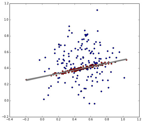
Here is a posterior predictive plot that shows it's recovering the linear regression: enter image description here

$\endgroup$
1
  • $\begingroup$ This is excellent. Thanks for all your work! I assume instead of using a pre-programmed parametric log-likelihood function for the noise and estimating its parameters I could also try to estimate something more general, e.g. fit a KDE? $\endgroup$
    – RoyalTS
    Commented Aug 19, 2014 at 14:15

Your Answer

By clicking “Post Your Answer”, you agree to our terms of service and acknowledge you have read our privacy policy.

Not the answer you're looking for? Browse other questions tagged or ask your own question.