The easiest way to do this in R is to use the bs (B-spline) function. Specifying a degree of 1 makes it piecewise linear. Here's an example, using different data since in your example, there's no dependence between x and y.
Generate some reproducible data
> set.seed(1234)
> x <- runif(150, -2, 3)
> y <- 7 * pnorm(x, 1, 0.7)^2 + rnorm(150, 0, .15)
Set up points where you want the slope to change
> knots <- c(-1,0,1,2) # interior ones only
Fit a model and plot the fitted values
> piecel.lm <- lm(y ~ bs(x, degree = 1, knots = knots, Boundary.knots = c(-2,3)))
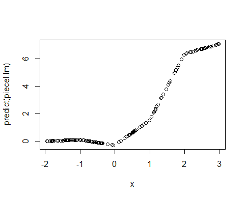
> plot(x, predict(piecel.lm))

(This shows that it is indeed piecewise linear. But to get it in more useful form, just figure out the abscissae and ordinates at the knots (including the end ones):
> absc <- (-2):3
> ord <- predict(piecel.lm, newdata = data.frame(x = absc))
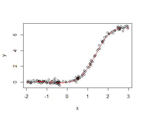
> plot(y ~ x)
> lines(ord ~ absc, col = "red")
> points(ord ~ absc, col = "red")

Additional comment:
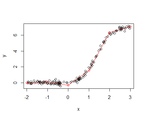
If your goal is simply to have something that'll fit the data better than a polynomial, I'd suggest a natural cubic spline, which you can get in much the same was using the ns function. You can evaluate it at any $x$ value using the predict function with newdata. Here is the natural spline fit to these data, using the same knots:
> spline.lm <- lm(y ~ ns(x, knots = knots, Boundary.knots = c(-2,3)))
> plot(y ~ x)
> xnew <- seq(-2, 3, by = .2)
> lines(xnew, predict(spline.lm, newdata = data.frame(x = xnew)), col = "red")
