Is rstan or my grid approximation incorrect: deciding between conflicting quantile estimates in Bayesian inference

Question

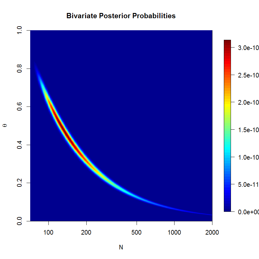
I have a model to achieve Bayesian estimates the population size $N$ and probability of detection $\theta$ in a binomial distribution solely based on the observed number of observed objects $y$: $$ p(N,\theta|y)\propto \frac{ \text{Bin}(y|N,\theta)}{N} $$ for $ \left\{N|N\in\mathbb{Z}\land N\ge \max(y)\right\}\times(0,1) $. For simplicity, we assume that $N$ is fixed at the same, unknown value for each $y_i$. In this example, $y=53,57,66,67,73$.

This model, when estimated in rstan, diverges from the results obtained from a grid approximation of the posterior. I'm trying to pin down why. (Interested readers might find that this question is a follow-on to my answer here.)

rstan Approximation

For reference, this is the rstan code.

raftery.model   <- "
    data{
        int     I;
        int     y[I];
    }
    parameters{
        real<lower=max(y)>  N;
        simplex[2]      theta;
    }
    transformed parameters{
    }
    model{
        vector[I]   Pr_y;

        for(i in 1:I){
            Pr_y[i] <-  binomial_coefficient_log(N, y[i])
                        +multiply_log(y[i],         theta[1])
                        +multiply_log((N-y[i]),     theta[2]);
        }
        increment_log_prob(sum(Pr_y));
        increment_log_prob(-log(N));            
    }
"
raft.data           <- list(y=c(53,57,66,67,72), I=5)
system.time(fit.test    <- stan(model_code=raftery.model, data=raft.data,iter=10))
system.time(fit     <- stan(fit=fit.test, data=raft.data,iter=10000,chains=5))

Note that I cast theta as a 2-simplex. This is just for simplicity. The quantity of interest is theta[1]; obviously theta[2] is superfluous information.

Additionally, $N$ is a real value (rstan only accepts real-valued parameters because it is a gradient method), so I wrote a real-valued binomial distribution.

Rstan results

            mean se_mean       sd   2.5%    25%    50%    75%   97.5% n_eff Rhat
N        1078.75  256.72 15159.79  94.44 148.28 230.61 461.63 4575.49  3487    1
theta[1]    0.29    0.00     0.19   0.01   0.14   0.27   0.42    0.67  2519    1
theta[2]    0.71    0.00     0.19   0.33   0.58   0.73   0.86    0.99  2519    1
lp__      -19.88    0.02     1.11 -22.89 -20.31 -19.54 -19.09  -18.82  3339    1

Grid Approximation

The grid approximation was produced as below. Memory constraints prevent me making a finer grid on my laptop.

theta   <- seq(0+1e-10,1-1e-10, len=1e3)
N       <- round(seq(72, 5000, len=1e3)); N[2]-N[1]
grid    <- expand.grid(N,theta)
y   <- c(53,57,66,67,72)
raftery.prob    <- function(x, z=y){
    N       <- x[1]
    theta   <- x[2]
    exp(sum(dbinom(z, size=N, prob=theta, log=T)))/N
}

post        <- matrix(apply(grid, 1, raftery.prob), nrow=length(N), ncol=length(theta),byrow=F)    
post.norm   <- post/sum(post)

I used the grid approximation to produce this display of the posterior density. We can see that the posterior is banana-shaped; this kind of posterior can be problematic for euclidian metric HMC. (The severity of the banana shape is actually suppressed here since $N$ is on the log scale.) If you think about the banana shape for a minute, you'll realize that it must lie on the line $\bar{y}=\theta N$. (Additionally, the grid approximation displayed in this graph is not normalized for reasons of clarity - else the banana is a little too narrow to clearly make out.)

Grid approximation results

do.call(cbind, lapply(c(0.025, .25, .5, .75, .975), function(quantile){
    approx(y=N, x=cumsum(rowSums(post.norm))/sum(post.norm), xout=quantile)
}))
  [,1]     [,2]     [,3]     [,4]     [,5]    
x 0.025    0.25     0.5      0.75     0.975   
y 92.55068 144.7091 226.7845 443.6359 2475.398

Discussion

The 97.5% quantile for $N$ is much larger in my rstan model than it is for the grid approximation, but its quantiles are similar to the grid approximation otherwise. I interpret this as indicating that the two methods are generally in agreement. I do not know how to interpret the discrepancy in the 97.5% quantile, though.

I've developed several possible explanations for what might be accounting for the divergence between the grid approximation and the results from rstan HMC-NUTS sampling, but I'm uncertain how to understand if one, both or neither explanation is correct.

1. Rstan is wrong and the grid is correct. The banana-shaped density is problematic for rstan, especially as $N$ drifts off towards $+\infty$, so these tail quantities are not trustworthy. We can see from the plot of the posterior over the grid that the tail is very sharp at larger values $N$.
2. Rstan is correct and the grid is wrong. The grid makes two approximations which may undermine the results. First, the grid is only a finite set of points over a subspace the posterior, so it is a rough approximation. Second, because it's a finite subspace, we're falsely declaring there to be 0 posterior probability over values $N$ larger than our largest grid value for $N$. Likewise, rstan is better at getting into the tails of the grid, so its tail quanitles are correct.

---

I needed more space to clarify a point from Juho's answer. If I understand correctly, we can integrate $\theta$ out of the posterior to obtain the beta-binomial distribution: $$ p(y|N,\alpha,\beta)={N\choose y} \frac{\text{Beta}(y+\alpha, N-y+\beta)}{\text{Beta}(\alpha,\beta)} $$

In our case, $\alpha=1$ and $\beta=1$ because we have a uniform prior on $\theta$. I believe that the posterior should then be $p(N|y)\propto N^{-1}\prod_{i=1}^K p(y_i|N,\alpha=1,\beta=1)$ where $K=\#(y)$ because $p(N)=N^{-1}$. But this appears to wildly diverge from Juho's answer. Where have I gone wrong?

Answer 1

Cliffs: Rstan seems to be (closer to) correct based on an approach that integrates $\theta$ out analytically and evaluates $P(N)P(y\mid N)$ in a rather big grid.

To get the posterior of $N$, it is actually possible to integrate $\theta$ out analytically: \begin{equation} P(y \mid N) = P(y_1 \mid N)\times P(y_2 \mid N,y_1)\times P(y_3 \mid N,y_1,y_2) \times \ldots P(y_K \mid N,y_1,\ldots,y_{K-1}) \end{equation} where $K$ is the length of $y$. Now, since $\theta$ has Beta prior (here $Beta(1,1)$) and Beta is conjugate to binomial, $\theta \mid N, y_1, \ldots, y_k$ also follows a Beta distribution. Therefore, the distribution of $y_{k+1} \mid N, y_1, \ldots, y_k$ is Beta-binomial for which a closed form expression of the probabilities exists in terms of the Gamma function. Therefore, we may evaluate $P(y\mid N)$ by computing the relevant parameters of the Beta-binomials and multiplying Beta-binomial probabilities. The following MATLAB code uses this approach to compute $P(N)P(y|N)$ for $N=72,\ldots,500000$ and normalizes to get the posterior.

%The data
y = [53 57 66 67 72];

%Initialize
maxN = 500000;
logp = zeros(1,maxN); %log prior + log likelihood
logp(1:71) = -inf; 

for N = 72:maxN
    %Prior
    logp(N) = -log(N);

    %y1 has uniform distribution
    logp(N) = logp(N) - log(N+1);    
    a = 1;
    b = 1;

    %Rest of the measurements 
    for j = 2:length(y);
        %Update beta parameters
        a = a + y(j-1);
        b = b + N - y(j-1);

        %Log predictive probability of y_j (see Wikipedia article)
        logp(N) = logp(N) + gammaln(N+1) - gammaln(y(j) + 1) - ... 
         gammaln(N - y(j) + 1) + gammaln(y(j) + a) +  ...
         gammaln(N - y(j) + b) - gammaln(N + a + b) ...
            + gammaln(a+b) - gammaln(a) - gammaln(b);

    end
end

%Get the posterior of N
pmf = exp(logp - max(logp));
pmf = pmf/sum(pmf);
cdf = cumsum(pmf);

%Evaluate quantiles of interest
disp(cdf(5000))  %0.9763
for percentile = [0.025 0.25 0.5 0.75 0.975]
    disp(find(cdf>=percentile,1,'first'))
end

The cdf at $N=100000$ is $0.9990$, so I guess maxN=500000 is enough, but one might want to investigate sensitivity to increasing the maximum $N$. The cdf at $N=5000$ is only $0.9763$ so your original grid indeed misses quite significant tail probability mass compared to the goal of finding the $0.975$ quantile. The quantiles I get are \begin{equation} \begin{array}{lllll} \textrm{Quantile} & 0.025 & 0.25 & 0.5 & 0.75 & 0.975 \\ N & 95 & 149 & 235 & 478 & 4750 \end{array} \end{equation}

Disclaimer: I did not test the code much, there may be errors (and obviously there could be numeric problems with this approach, too). However, the obtained quantiles are quite close to the Rstan results, so I am rather confident.