563
$\begingroup$

In the definition of standard deviation, why do we have to square the difference from the mean to get the mean (E) and take the square root back at the end? Can't we just simply take the absolute value of the difference instead and get the expected value (mean) of those, and wouldn't that also show the variation of the data? The number is going to be different from square method (the absolute-value method will be smaller), but it should still show the spread of data. Anybody know why we take this square approach as a standard?

The definition of standard deviation:

$\sigma = \sqrt{E\left[\left(X - \mu\right)^2\right]}.$

Can't we just take the absolute value instead and still be a good measurement?

$\sigma = E\left[|X - \mu|\right]$

$\endgroup$
26
  • 40
    $\begingroup$ In a way, the measurement you proposed is widely used in case of error (model quality) analysis -- then it is called MAE, "mean absolute error". $\endgroup$
    – user88
    Commented Jul 19, 2010 at 21:30
  • 10
    $\begingroup$ In accepting an answer it seems important to me that we pay attention to whether the answer is circular. The normal distribution is based on these measurements of variance from squared error terms, but that isn't in and of itself a justification for using (X-M)^2 over |X-M|. $\endgroup$ Commented Jul 20, 2010 at 7:59
  • 76
    $\begingroup$ Every answer offered so far is circular. They focus on ease of mathematical calculations (which is nice but by no means fundamental) or on properties of the Gaussian (Normal) distribution and OLS. Around 1800 Gauss started with least squares and variance and from those derived the Normal distribution--there's the circularity. A truly fundamental reason that has not been invoked in any answer yet is the unique role played by the variance in the Central Limit Theorem. Another is the importance in decision theory of minimizing quadratic loss. $\endgroup$
    – whuber
    Commented Sep 13, 2013 at 15:28
  • 12
    $\begingroup$ Taleb makes the case at Edge.org for retiring standard deviation and using mean absolute deviation. $\endgroup$ Commented Jun 2, 2015 at 10:38
  • 4
    $\begingroup$ @A.S. Sure--I have answered this question in some detail at stats.stackexchange.com/a/3904. Briefly, there are infinitely many such functionals--but they must all asymptotically converge to the variance. $\endgroup$
    – whuber
    Commented Jan 27, 2016 at 20:03

23 Answers 23

261
$\begingroup$

If the goal of the standard deviation is to summarise the spread of a symmetrical data set (i.e. in general how far each datum is from the mean), then we need a good method of defining how to measure that spread.

The benefits of squaring include:

  • Squaring always gives a non-negative value, so the sum will always be zero or higher.
  • Squaring emphasizes larger differences, a feature that turns out to be both good and bad (think of the effect outliers have).

Squaring however does have a problem as a measure of spread and that is that the units are all squared, whereas we might prefer the spread to be in the same units as the original data (think of squared pounds, squared dollars, or squared apples). Hence the square root allows us to return to the original units.

I suppose you could say that absolute difference assigns equal weight to the spread of data whereas squaring emphasises the extremes. Technically though, as others have pointed out, squaring makes the algebra much easier to work with and offers properties that the absolute method does not (for example, the variance is equal to the expected value of the square of the distribution minus the square of the mean of the distribution)

It is important to note however that there's no reason you couldn't take the absolute difference if that is your preference on how you wish to view 'spread' (sort of how some people see 5% as some magical threshold for $p$-values, when in fact it is situation dependent). Indeed, there are in fact several competing methods for measuring spread.

My view is to use the squared values because I like to think of how it relates to the Pythagorean Theorem of Statistics: $c = \sqrt{a^2 + b^2}$ …this also helps me remember that when working with independent random variables, variances add, standard deviations don't. But that's just my personal subjective preference which I mostly only use as a memory aid, feel free to ignore this paragraph.

An interesting analysis can be read here:

$\endgroup$
11
  • 119
    $\begingroup$ "Squaring always gives a positive value, so the sum will not be zero." and so does absolute values. $\endgroup$ Commented Jul 22, 2010 at 9:54
  • 45
    $\begingroup$ @robin girard: That is correct, hence why I preceded that point with "The benefits of squaring include". I wasn't implying that anything about absolute values in that statement. I take your point though, I'll consider removing/rephrasing it if others feel it is unclear. $\endgroup$ Commented Jul 22, 2010 at 13:19
  • 19
    $\begingroup$ Much of the field of robust statistics is an attempt to deal with the excessive sensitivity to outliers that that is a consequence of choosing the variance as a measure of data spread (technically scale or dispersion). en.wikipedia.org/wiki/Robust_statistics $\endgroup$
    – Thylacoleo
    Commented Aug 13, 2010 at 5:15
  • 10
    $\begingroup$ The article linked to in the answer is a god send. $\endgroup$
    – traggatmot
    Commented Mar 19, 2015 at 7:27
  • 5
    $\begingroup$ I think the paragraph about Pythagoras is spot on. You can think of the error as a vector in $n$ dimensions, with $n$ being the number of samples. The size in each dimension is the difference from the mean for that sample. $[(x_1-\mu), (x_2-\mu), (x_3-\mu), ...]$ The length of that vector (Pythagoras) is the root of summed squares, i.e. the standard deviation. $\endgroup$ Commented Sep 30, 2017 at 9:39
162
$\begingroup$

The squared difference has nicer mathematical properties; it's continuously differentiable (nice when you want to minimize it), it's a sufficient statistic for the Gaussian distribution, and it's (a version of) the L2 norm which comes in handy for proving convergence and so on.

The mean absolute deviation (the absolute value notation you suggest) is also used as a measure of dispersion, but it's not as "well-behaved" as the squared error.

$\endgroup$
8
  • 5
    $\begingroup$ said "it's continuously differentiable (nice when you want to minimize it)" do you mean that the absolute value is difficult to optimize ? $\endgroup$ Commented Jul 23, 2010 at 21:40
  • 36
    $\begingroup$ @robin: while the absolute value function is continuous everywhere, its first derivative is not (at x=0). This makes analytical optimization more difficult. $\endgroup$
    – Vince
    Commented Jul 23, 2010 at 23:59
  • 12
    $\begingroup$ Yes, but finding the actual number you want, rather than just a descriptor of it, is easier under squared error loss. Consider the 1 dimension case; you can express the minimizer of the squared error by the mean: O(n) operations and closed form. You can express the value of the absolute error minimizer by the median, but there's not a closed-form solution that tells you what the median value is; it requires a sort to find, which is something like O(n log n). Least squares solutions tend to be a simple plug-and-chug type operation, absolute value solutions usually require more work to find. $\endgroup$
    – Rich
    Commented Jul 24, 2010 at 9:10
  • 8
    $\begingroup$ @Rich: Both the variance and the median can be found in linear time, and of course no faster. Median does not require sorting. $\endgroup$
    – Neil G
    Commented May 19, 2014 at 20:02
  • 5
    $\begingroup$ @JeromeBaum: en.wikipedia.org/wiki/Median_of_medians $\endgroup$
    – Neil G
    Commented Dec 27, 2014 at 4:11
102
$\begingroup$

One way you can think of this is that standard deviation is similar to a "distance from the mean".

Compare this to distances in euclidean space - this gives you the true distance, where what you suggested (which, btw, is the absolute deviation) is more like a manhattan distance calculation.

$\endgroup$
5
  • 26
    $\begingroup$ Nice analogy of euclidean space! $\endgroup$
    – c4il
    Commented Jul 19, 2010 at 21:38
  • 4
    $\begingroup$ Except that in one dimension the $l_1$ and $l_2$ norm are the same thing, aren't they? $\endgroup$
    – naught101
    Commented Mar 29, 2012 at 5:20
  • 6
    $\begingroup$ @naught101: It's not one dimension, but rather $n$ dimensions where $n$ is the number of samples. The standard deviation and the absolute deviation are (scaled) $l_2$ and $l_1$ distances respectively, between the two points $(x_1, x_2, \dots, x_n)$ and $(\mu, \mu, \dots, \mu)$ where $\mu$ is the mean. $\endgroup$ Commented Nov 16, 2012 at 7:21
  • 1
    $\begingroup$ This should be modified as minimum distance from the mean. It's essentially a Pythagorean equation. $\endgroup$
    – John
    Commented Nov 21, 2014 at 16:40
  • $\begingroup$ Related datascience.stackexchange.com/a/20234/159228 $\endgroup$ Commented Jan 25 at 16:13
75
$\begingroup$

The reason that we calculate standard deviation instead of absolute error is that we are assuming error to be normally distributed. It's a part of the model.

Suppose you were measuring very small lengths with a ruler, then standard deviation is a bad metric for error because you know you will never accidentally measure a negative length. A better metric would be one to help fit a Gamma distribution to your measurements:

$\log(E(x)) - E(\log(x))$

Like the standard deviation, this is also non-negative and differentiable, but it is a better error statistic for this problem.

$\endgroup$
12
  • 6
    $\begingroup$ I like your answer. The sd is not always the best statistic. $\endgroup$ Commented Nov 25, 2010 at 3:03
  • 5
    $\begingroup$ Great counter-example as to when the standard deviation is not the best way to think of fluctuation sizes. $\endgroup$
    – Hbar
    Commented May 13, 2014 at 2:49
  • $\begingroup$ Shouldn't you have an opposite sign on the quantity to yield a positive measure - using a convex $-log x$ instead of concave $\log x$? $\endgroup$
    – A.S.
    Commented Jan 27, 2016 at 20:58
  • $\begingroup$ @A.S. No, it is already always positive. It is zero when all the samples $x$ are equal, and otherwise its magnitude measures variation. $\endgroup$
    – Neil G
    Commented Jan 27, 2016 at 22:21
  • 1
    $\begingroup$ @GENIVI-LEARNER yes. This is what I mean. After all you want the best model. $\endgroup$
    – Neil G
    Commented Apr 19, 2020 at 18:51
32
$\begingroup$

The answer that best satisfied me is that it falls out naturally from the generalization of a sample to n-dimensional euclidean space. It's certainly debatable whether that's something that should be done, but in any case:

Assume your $n$ measurements $X_i$ are each an axis in $\mathbb R^n$. Then your data $x_i$ define a point $\bf x$ in that space. Now you might notice that the data are all very similar to each other, so you can represent them with a single location parameter $\mu$ that is constrained to lie on the line defined by $X_i=\mu$. Projecting your datapoint onto this line gets you $\hat\mu=\bar x$, and the distance from the projected point $\hat\mu\bf 1$ to the actual datapoint is $\sqrt{\frac{n-1} n}\hat\sigma=\|\bf x-\hat\mu\bf 1\|$.

This approach also gets you a geometric interpretation for correlation, $\hat\rho=\cos \angle(\vec{\bf\tilde x},\vec{\bf\tilde y})$.

$\endgroup$
9
  • 11
    $\begingroup$ This is correct and appealing. However, in the end it appears only to rephrase the question without actually answering it: namely, why should we use the Euclidean (L2) distance? $\endgroup$
    – whuber
    Commented Nov 24, 2010 at 21:07
  • 26
    $\begingroup$ @sesqu Standard deviations did not become commonplace until Gauss in 1809 derived his eponymous deviation using squared error, rather than absolute error, as a starting point. However, what pushed them over the top (I believe) was Galton's regression theory (at which you hint) and the ability of ANOVA to decompose sums of squares--which amounts to a restatement of the Pythagorean Theorem, a relationship enjoyed only by the L2 norm. Thus the SD became a natural omnibus measure of spread advocated in Fisher's 1925 "Statistical Methods for Research Workers" and here we are, 85 years later. $\endgroup$
    – whuber
    Commented Nov 24, 2010 at 21:56
  • 16
    $\begingroup$ (+1) Continuing in @whuber's vein, I would bet that had Student published a paper in 1908 entitled, "Probable Error of the Mean - Hey, Guys, Check Out That MAE in the Denominator!" then statistics would have an entirely different face by now. Of course, he didn't publish a paper like that, and of course he couldn't have, because the MAE doesn't boast all the nice properties that S^2 has. One of them (related to Student) is its independence of the mean (in the normal case), which of course is a restatement of orthogonality, which gets us right back to L2 and the inner product. $\endgroup$
    – user1108
    Commented Nov 25, 2010 at 3:38
  • 3
    $\begingroup$ This answer was thought-provoking and I think my preferred way of viewing it. In 1-D it's hard to understand why squaring the difference is seen as better. But in multiple dimensions (or even just 2) one can easily see that Euclidean distance (squaring) is preferable to Manhattan distance (sum of absolute value of differences). $\endgroup$
    – thecity2
    Commented Jun 7, 2016 at 21:25
  • 3
    $\begingroup$ @whuber Can you please explain what "the line defined by Xᵢ = μ" means? Is it the line passing through the origin and the point (μ, μ, ..., μ)? Also, where can I read more about this? $\endgroup$ Commented Mar 19, 2019 at 7:15
22
$\begingroup$

Squaring the difference from the mean has a couple of reasons.

  • Variance is defined as the 2nd moment of the deviation (the R.V here is $(x-\mu)$) and thus the square as moments are simply the expectations of higher powers of the random variable.

  • Having a square as opposed to the absolute value function gives a nice continuous and differentiable function (absolute value is not differentiable at 0) - which makes it the natural choice, especially in the context of estimation and regression analysis.

  • The squared formulation also naturally falls out of parameters of the Normal Distribution.

$\endgroup$
19
$\begingroup$

Just so people know, there is a Math Overflow question on the same topic.

Why-is-it-so-cool-to-square-numbers-in-terms-of-finding-the-standard-deviation

The take away message is that using the square root of the variance leads to easier maths. A similar response is given by Rich and Reed above.

$\endgroup$
2
  • 7
    $\begingroup$ 'Easier math' isn't an essential requirement when we want our formulas and values to more truly reflect a given set of data. Computers do all the hard work anyway. $\endgroup$
    – Dan W
    Commented Jul 31, 2015 at 5:26
  • 6
    $\begingroup$ Defining pi as 3.14 makes math easier, but that doesn't make it right. $\endgroup$
    – James
    Commented Nov 28, 2015 at 3:29
19
$\begingroup$

$\newcommand{\var}{\operatorname{var}}$ Variances are additive: for independent random variables $X_1,\ldots,X_n$, $$ \var(X_1+\cdots+X_n)=\var(X_1)+\cdots+\var(X_n). $$

Notice what this makes possible: Say I toss a fair coin 900 times. What's the probability that the number of heads I get is between 440 and 455 inclusive? Just find the expected number of heads ($450$), and the variance of the number of heads ($225=15^2$), then find the probability with a normal (or Gaussian) distribution with expectation $450$ and standard deviation $15$ is between $439.5$ and $455.5$. Abraham de Moivre did this with coin tosses in the 18th century, thereby first showing that the bell-shaped curve is worth something.

$\endgroup$
4
  • 2
    $\begingroup$ Are mean absolute deviations not additive in the same way as variances? $\endgroup$ Commented Feb 9, 2013 at 23:30
  • 7
    $\begingroup$ No, they're not. $\endgroup$ Commented Feb 10, 2013 at 18:14
  • 1
    $\begingroup$ Why arnt mean absolute deviations not additive? Can you please point to a reference? $\endgroup$ Commented Apr 19, 2020 at 18:13
  • 3
    $\begingroup$ @GENIVI-LEARNER : You can verify that m.a.d. is not additive just by computing a few examples. But I'll see if I can find something on that. $\endgroup$ Commented Apr 20, 2020 at 18:50
16
$\begingroup$

Yet another reason (in addition to the excellent ones above) comes from Fisher himself, who showed that the standard deviation is more "efficient" than the absolute deviation. Here, efficient has to do with how much a statistic will fluctuate in value on different samplings from a population. If your population is normally distributed, the standard deviation of various samples from that population will, on average, tend to give you values that are pretty similar to each other, whereas the absolute deviation will give you numbers that spread out a bit more. Now, obviously this is in ideal circumstances, but this reason convinced a lot of people (along with the math being cleaner), so most people worked with standard deviations.

$\endgroup$
3
  • 8
    $\begingroup$ Your argument depends on the data being normally distributed. If we assume the population to have a "double exponential" distribution, then the absolute deviation is more efficient (in fact it is a sufficient statistic for the scale) $\endgroup$ Commented Jul 16, 2011 at 5:08
  • 9
    $\begingroup$ Yes, as I stated, "if your population is normally distributed." $\endgroup$
    – Eric Suh
    Commented Sep 8, 2011 at 19:49
  • 1
    $\begingroup$ Besides assuming normal distribution Fisher proof assumes error-free measurements. With small errors like 1% the situation inverts and the average absolute deviation is more efficient than the standard deviation $\endgroup$
    – juanrga
    Commented Aug 6, 2017 at 10:51
11
$\begingroup$

Estimating the standard deviation of a distribution requires to choose a distance.
Any of the following distance can be used:

$$d_n((X)_{i=1,\ldots,I},\mu)=\left(\sum | X-\mu|^n\right)^{1/n}$$

We usually use the natural euclidean distance ($n=2$), which is the one everybody uses in daily life. The distance that you propose is the one with $n=1$.
Both are good candidates but they are different.

One could decide to use $n=3$ as well.

I am not sure that you will like my answer, my point contrary to others is not to demonstrate that $n=2$ is better. I think that if you want to estimate the standard deviation of a distribution, you can absolutely use a different distance.

$\endgroup$
1
  • $\begingroup$ So, if you map the n values (k_i-mean) to a single point in n-dimensional space, the standard deviation is the length of the corresponding vector, scaled by 1/sqrt(n). $\endgroup$ Commented Feb 21, 2020 at 13:06
11
$\begingroup$

Why square the difference instead of taking the absolute value in standard deviation?

We square the difference of the x's from the mean because the Euclidean distance proportional to the square root of the degrees of freedom (number of x's, in a population measure) is the best measure of dispersion.

That is, when the x's have zero mean, $\mu = 0$:

$$ \sigma = \sqrt{\frac{\displaystyle\sum_{i=1}^{n}(x_i - \mu)^2} {n}} = \frac{\sqrt{\displaystyle\sum_{i=1}^{n}(x_i)^2}} {\sqrt{n}} = \frac{distance}{\sqrt{n}} $$

The square root of the sum of squares is the $n$-dimensional distance from the mean to the point in the $n$ dimensional space denoted by each data point.

Calculating distance

What's the distance from point 0 to point 5?

  • $5-0 = 5$,
  • $|0-5| = 5$, and
  • $\sqrt{5^2} = 5$

Yes, that's trivial because it's a single dimension.

How about the distance from point (0, 0) to point (3, 4)?

If we can only go in 1 dimension at a time (like in city blocks) then we just add the numbers up. (This is sometimes known as the Manhattan distance).

But what about going in two dimensions at once? Then (by the Pythagorean theorem we all learned in high school), we square the distance in each dimension, sum the squares, and then take the square root to find the distance from the origin to the point.

$$ \sqrt{3^2 + 4^2} = \sqrt{25} = 5 $$

Visually (see the markdown source of the answer for the code to generate):
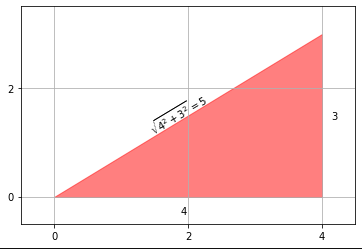
graph demonstrating 3 squared plus 4 squared = 5 squared

Calculating distance in higher dimensions

Now let's consider the 3 dimensional case, for example, how about the distance from point (0, 0, 0) to point (2, 2, 1)?

This is just

$$ \sqrt{\sqrt{2^2 + 2^2}^2 + 1^2} = \sqrt{2^2 + 2^2 + 1^2} = \sqrt9 = 3 $$

because the distance for the first two x's forms the leg for computing the total distance with the final x.

$$ \sqrt{\sqrt{x_1^2 + x_2^2}^2 + x_3^2} = \sqrt{x_1^2 + x_2^2 + x_3^2} $$

Demonstrated visually:
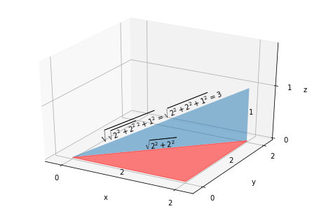
graph

We can continue to extend the rule of squaring each dimension's distance, this generalizes to what we call a Euclidean distance, for orthogonal measurements in $n$-dimensional space, like so:

$$ distance = \sqrt{ \sum\nolimits_{i=1}^n{x_i^2} } $$

and so the sum of orthogonal squares is the squared distance:

$$ distance^2 = \sum_{i=1}^n{x_i^2} $$

What makes a measurement orthogonal (or at right angles) to another? The condition is that there is no relationship between the two measurements. We would look for these measurements to be independent and individually distributed, (i.i.d.).

Variance

Now recall the formula for population variance (from which we'll get the standard deviation):

$$ \sigma^2 = \frac{\displaystyle\sum_{i=1}^{n}(x_i - \mu)^2} {n} $$

If we've already centered the data at 0 by subtracting the mean, we have:

$$ \sigma^2 = \frac{\displaystyle\sum_{i=1}^{n}(x_i)^2} {n} $$

So we see the variance is just the squared distance, or $distance^2$ (see above), divided by the number of degrees of freedom (the number of dimensions on which the variables are free to vary). This is also the average contribution to $distance^2$ per measurement. "Mean squared variance" would also be an appropriate term.

Standard Deviation

Then we have the standard deviation, which is just the square root of the variance:

$$ \sigma = \sqrt{\frac{\displaystyle\sum_{i=1}^{n}(x_i - \mu)^2} {n}} $$

Which is equivalently, the distance, divided by the square root of the degrees of freedom:

$$ \sigma = \frac{\sqrt{\displaystyle\sum_{i=1}^{n}(x_i)^2}} {\sqrt{n}} $$

Mean Absolute Deviation

Mean Absolute Deviation (MAD), is a measure of dispersion that uses the Manhattan distance, or the sum of absolute values of the differences from the mean.

$$ MAD = \frac{\displaystyle\sum_{i=1}^{n}|x_i - \mu|} {n} $$

Again, assuming the data is centered (the mean subtracted) we have the Manhattan distance divided by the number of measurements:

$$ MAD = \frac{\displaystyle\sum_{i=1}^{n}|x_i|} {n} $$

Discussion

  • The mean absolute deviation is about .8 times (actually $\sqrt{2/\pi}$) the size of the standard deviation for a normally distributed dataset.
  • Regardless of the distribution, the mean absolute deviation is less than or equal to the standard deviation. MAD understates the dispersion of a data set with extreme values, relative to standard deviation.
  • Mean Absolute Deviation is more robust to outliers (i.e. outliers do not have as great an effect on the statistic as they do on standard deviation.
  • Geometrically speaking, if the measurements are not orthogonal to each other (i.i.d.) - for example, if they were positively correlated, mean absolute deviation would be a better descriptive statistic than standard deviation, which relies on Euclidean distance (although this is usually considered fine).

This table reflects the above information in a more concise way:

$$ \begin{array}{lll} & MAD & \sigma \\ \hline size & \le \sigma & \ge MAD \\ size, \sim N & .8 \times \sigma & 1.25 \times MAD \\ outliers & robust & influenced \\ not\ i.i.d. & robust & ok \end{array} $$

Comments:

Do you have a reference for "mean absolute deviation is about .8 times the size of the standard deviation for a normally distributed dataset"? The simulations I'm running show this to be incorrect.

Here's 10 simulations of one million samples from the standard normal distribution:

>>> from numpy.random import standard_normal
>>> from numpy import mean, absolute
>>> for _ in range(10):
...     array = standard_normal(1_000_000)
...     print(numpy.std(array), mean(absolute(array - mean(array))))
... 
0.9999303226807994 0.7980634269273035
1.001126461808081 0.7985832977798981
0.9994247275533893 0.7980171649802613
0.9994142105335478 0.7972367136320848
1.0001188211817726 0.798021564315937
1.000442654481297 0.7981845236910842
1.0001537518728232 0.7975554993742403
1.0002838369191982 0.798143108250063
0.9999060114455384 0.797895284109523
1.0004871065680165 0.798726062813422

Conclusion

We prefer the squared differences when calculating a measure of dispersion because we can exploit the Euclidean distance, which gives us a better discriptive statistic of the dispersion. When there are more relatively extreme values, the Euclidean distance accounts for that in the statistic, whereas the Manhattan distance gives each measurement equal weight.

$\endgroup$
0
10
$\begingroup$

I think the contrast between using absolute deviations and squared deviations becomes clearer once you move beyond a single variable and think about linear regression. There's a nice discussion at http://en.wikipedia.org/wiki/Least_absolute_deviations, particularly the section "Contrasting Least Squares with Least Absolute Deviations" , which links to some student exercises with a neat set of applets at http://www.math.wpi.edu/Course_Materials/SAS/lablets/7.3/73_choices.html .

To summarise, least absolute deviations is more robust to outliers than ordinary least squares, but it can be unstable (small change in even a single datum can give big change in fitted line) and doesn't always have a unique solution - there can be a whole range of fitted lines. Also least absolute deviations requires iterative methods, while ordinary least squares has a simple closed-form solution, though that's not such a big deal now as it was in the days of Gauss and Legendre, of course.

$\endgroup$
1
  • $\begingroup$ the "unique solution" argument is quite weak, it really means there is more than one value well supported by the data. Additionally, penalisation of the coefficients, such as L2, will resolve the uniqueness problem, and the stability problem to a degree as well. $\endgroup$ Commented Jul 4, 2014 at 11:13
10
$\begingroup$

In many ways, the use of standard deviation to summarize dispersion is jumping to a conclusion. You could say that SD implicitly assumes a symmetric distribution because of its equal treatment of distance below the mean as of distance above the mean. The SD is surprisingly difficult to interpret to non-statisticians. One could argue that Gini's mean difference has broader application and is significantly more interpretable. It does not require one to declare their choice of a measure of central tendency as the use of SD does for the mean. Gini's mean difference is the average absolute difference between any two different observations. Besides being robust and easy to interpret it happens to be 0.98 as efficient as SD if the distribution were actually Gaussian.

$\endgroup$
2
  • 3
    $\begingroup$ Just to add to @Frank's suggestion on Gini, there's a nice paper here: projecteuclid.org/download/pdf_1/euclid.ss/1028905831 It goes over various measures of dispersion and also give an informative historical perspective. $\endgroup$ Commented May 14, 2014 at 17:06
  • 5
    $\begingroup$ I like these ideas too, but there's a less well known parallel definition of the variance (and thus the SD) that makes no reference to means as location parameters. The variance is half the mean square over all the pairwise differences between values, just as the Gini mean difference is based on the absolute values of all the pairwise difference. $\endgroup$
    – Nick Cox
    Commented Oct 21, 2014 at 23:46
9
$\begingroup$

There are many reasons; probably the main is that it works well as parameter of normal distribution.

$\endgroup$
3
  • 4
    $\begingroup$ I agree. Standard deviation is the right way to measure dispersion if you assume normal distribution. And a lot of distributions and real data are an approximately normal. $\endgroup$ Commented Jul 20, 2010 at 14:40
  • 2
    $\begingroup$ I don't think you should say "natural parameter": the natural parameters of the normal distribution are mean and mean times precision. (en.wikipedia.org/wiki/Natural_parameter) $\endgroup$
    – Neil G
    Commented Mar 12, 2012 at 7:40
  • 1
    $\begingroup$ @NeilG Good point; I was thinking about "casual" meaning here. I'll think about some better word. $\endgroup$
    – user88
    Commented Mar 12, 2012 at 10:41
8
$\begingroup$

"Why square the difference" instead of "taking absolute value"? To answer very exactly, there is literature that gives the reasons it was adopted and the case for why most of those reasons do not hold. "Can't we simply take the absolute value...?". I am aware of literature in which the answer is yes it is being done and doing so is argued to be advantageous.

Author Gorard states, first, using squares was previously adopted for reasons of simplicity of calculation but that those original reasons no longer hold. Gorard states, second, that OLS was adopted because Fisher found that results in samples of analyses that used OLS had smaller deviations than those that used absolute differences (roughly stated). Thus, it would seem that OLS may have benefits in some ideal circumstances; however, Gorard proceeds to note that there is some consensus (and he claims Fisher agreed) that under real world conditions (imperfect measurement of observations, non-uniform distributions, studies of a population without inference from a sample), using squares is worse than absolute differences.

Gorard's response to your question "Can't we simply take the absolute value of the difference instead and get the expected value (mean) of those?" is yes. Another advantage is that using differences produces measures (measures of errors and variation) that are related to the ways we experience those ideas in life. Gorard says imagine people who split the restaurant bill evenly and some might intuitively notice that that method is unfair. Nobody there will square the errors; the differences are the point.

Finally, using absolute differences, he notes, treats each observation equally, whereas by contrast squaring the differences gives observations predicted poorly greater weight than observations predicted well, which is like allowing certain observations to be included in the study multiple times. In summary, his general thrust is that there are today not many winning reasons to use squares and that by contrast using absolute differences has advantages.

References:

$\endgroup$
0
6
$\begingroup$

It depends on what you are talking about when you say "spread of the data". To me this could mean two things:

  1. The width of a sampling distribution
  2. The accuracy of a given estimate

For point 1) there is no particular reason to use the standard deviation as a measure of spread, except for when you have a normal sampling distribution. The measure $E(|X-\mu|)$ is a more appropriate measure in the case of a Laplace Sampling distribution. My guess is that the standard deviation gets used here because of intuition carried over from point 2). Probably also due to the success of least squares modelling in general, for which the standard deviation is the appropriate measure. Probably also because calculating $E(X^2)$ is generally easier than calculating $E(|X|)$ for most distributions.

Now, for point 2) there is a very good reason for using the variance/standard deviation as the measure of spread, in one particular, but very common case. You can see it in the Laplace approximation to a posterior. With Data $D$ and prior information $I$, write the posterior for a parameter $\theta$ as:

$$p(\theta\mid DI)=\frac{\exp\left(h(\theta)\right)}{\int \exp\left(h(t)\right)\,dt}\;\;\;\;\;\;h(\theta)\equiv\log[p(\theta\mid I)p(D\mid\theta I)]$$

I have used $t$ as a dummy variable to indicate that the denominator does not depend on $\theta$. If the posterior has a single well rounded maximum (i.e. not too close to a "boundary"), we can taylor expand the log probability about its maximum $\theta_\max$. If we take the first two terms of the taylor expansion we get (using prime for differentiation):

$$h(\theta)\approx h(\theta_\max)+(\theta_\max-\theta)h'(\theta_\max)+\frac{1}{2}(\theta_\max-\theta)^{2}h''(\theta_\max)$$

But we have here that because $\theta_\max$ is a "well rounded" maximum, $h'(\theta_\max)=0$, so we have:

$$h(\theta)\approx h(\theta_\max)+\frac{1}{2}(\theta_\max-\theta)^{2}h''(\theta_\max)$$

If we plug in this approximation we get:

$$p(\theta\mid DI)\approx\frac{\exp\left(h(\theta_\max)+\frac{1}{2}(\theta_\max-\theta)^{2}h''(\theta_\max)\right)}{\int \exp\left(h(\theta_\max)+\frac{1}{2}(\theta_\max-t)^{2}h''(\theta_\max)\right)\,dt}$$

$$=\frac{\exp\left(\frac{1}{2}(\theta_\max-\theta)^{2}h''(\theta_\max)\right)}{\int \exp\left(\frac{1}{2}(\theta_\max-t)^{2}h''(\theta_\max)\right)\,dt}$$

Which, but for notation is a normal distribution, with mean equal to $E(\theta\mid DI)\approx\theta_\max$, and variance equal to

$$V(\theta\mid DI)\approx \left[-h''(\theta_\max)\right]^{-1}$$

($-h''(\theta_\max)$ is always positive because we have a well rounded maximum). So this means that in "regular problems" (which is most of them), the variance is the fundamental quantity which determines the accuracy of estimates for $\theta$. So for estimates based on a large amount of data, the standard deviation makes a lot of sense theoretically - it tells you basically everything you need to know. Essentially the same argument applies (with same conditions required) in multi-dimensional case with $h''(\theta)_{jk}=\frac{\partial h(\theta)}{\partial \theta_j \, \partial \theta_k}$ being a Hessian matrix. The diagonal entries are also essentially variances here too.

The frequentist using the method of maximum likelihood will come to essentially the same conclusion because the MLE tends to be a weighted combination of the data, and for large samples the Central Limit Theorem applies and you basically get the same result if we take $p(\theta\mid I)=1$ but with $\theta$ and $\theta_\max$ interchanged: $$p(\theta_\max\mid\theta)\approx N\left(\theta,\left[-h''(\theta_\max)\right]^{-1}\right)$$ (see if you can guess which paradigm I prefer :P ). So either way, in parameter estimation the standard deviation is an important theoretical measure of spread.

$\endgroup$
5
$\begingroup$

When adding random variables, their variances add, for all distributions. Variance (and therefore standard deviation) is a useful measure for almost all distributions, and is in no way limited to gaussian (aka "normal") distributions. That favors using it as our error measure. Lack of uniqueness is a serious problem with absolute differences, as there are often an infinite number of equal-measure "fits", and yet clearly the "one in the middle" is most realistically favored. Also, even with today's computers, computational efficiency matters. I work with large data sets, and CPU time is important. However, there is no single absolute "best" measure of residuals, as pointed out by some previous answers. Different circumstances sometimes call for different measures.

$\endgroup$
3
  • 4
    $\begingroup$ I remain unconvinced that variances are very useful for asymmetric distributions. $\endgroup$ Commented Oct 22, 2014 at 12:58
  • 1
    $\begingroup$ What about a pair of "semi-variances", one upward, one downward? $\endgroup$ Commented Oct 26, 2018 at 18:13
  • $\begingroup$ Variances only add for independent random variables. $\endgroup$
    – cdalitz
    Commented May 17, 2022 at 13:45
4
$\begingroup$

Because squares can allow use of many other mathematical operations or functions more easily than absolute values.

Example: squares can be integrated, differentiated, can be used in trigonometric, logarithmic and other functions, with ease.

$\endgroup$
1
  • 2
    $\begingroup$ I wonder if there is a self fulfilling profecy here. We get $\endgroup$ Commented Mar 13, 2012 at 12:04
3
$\begingroup$

Naturally you can describe dispersion of a distribution in any way meaningful (absolute deviation, quantiles, etc.).

One nice fact is that the variance is the second central moment, and every distribution is uniquely described by its moments if they exist. Another nice fact is that the variance is much more tractable mathematically than any comparable metric. Another fact is that the variance is one of two parameters of the normal distribution for the usual parametrization, and the normal distribution only has 2 non-zero central moments which are those two very parameters. Even for non-normal distributions it can be helpful to think in a normal framework.

As I see it, the reason the standard deviation exists as such is that in applications the square-root of the variance regularly appears (such as to standardize a random varianble), which necessitated a name for it.

$\endgroup$
2
  • 2
    $\begingroup$ If I recall correctly, isn't the log-normal distribution not uniquely defined by its moments. $\endgroup$ Commented Apr 10, 2014 at 13:38
  • 2
    $\begingroup$ @probabilityislogic, indeed, that is true, see en.wikipedia.org/wiki/Log-normal_distribution in the section "Characteristic function and moment generating function". $\endgroup$ Commented Aug 2, 2015 at 18:45
3
$\begingroup$

A different and perhaps more intuitive approach is when you think about linear regression vs. median regression.

Suppose our model is that $\mathbb{E}(y|x) = x\beta$. Then we find b by minimisize the expected squared residual, $\beta = \arg \min_b \mathbb{E} (y - x b)^2$.

If instead our model is that Median$(y|x) = x\beta$, then we find our parameter estimates by minimizing the absolute residuals, $\beta = \arg \min_b \mathbb{E} |y - x b|$.

In other words, whether to use absolute or squared error depends on whether you want to model the expected value or the median value.

If the distribution, for example, displays skewed heteroscedasticity, then there is a big difference in how the slope of the expected value of $y$ changes over $x$ to how the slope is for the median value of $y$.

Koenker and Hallock have a nice piece on quantile regression, where median regression is a special case.

$\endgroup$
2
$\begingroup$

This is an old thread, but most answers focus on analytical simplicity, which IMO is a weak argument in times of computers (although numerical stability might be an issue when using absolute values in optimization routines). Here are some more fundamental arguments in favor of the variance.

  1. The statistical mean minimizes the variance (MSE), i.e. $$\overline{x}=\arg\min_m\left\{\sum_{1=1}^n(x_i-m)^2\right\}$$ whereas the mean absolute error (MAE) is minimized by the median: $$x_{med}=\arg\min_m\left\{\sum_{1=1}^n|x_i-m|\right\}$$ A dispersion measure that uses the absolute distances should thus be based on the median and not the mean.
  2. Variances are additive for independent variables, i.e. $Var(X+Y)=Var(X)+Var(Y)$. The same does not hold for the mean absolute deviation (this was already mentioned by @eric-l-michelsen).
  3. For mean absolute deviations, there is no approximation rule for error propagation (propagation of uncertainty). For the variance, there is Gauss' law $$Var(f(X_1,X_2,\ldots,X_k))\approx \sum_{i=1}^k \left(\left.\frac{\partial f}{\partial X_i}\right|_{E(X)}\right)^2 Var(X_i)$$
  4. The variance nicely generalizes to unsymmetric distributions, because it is the second central moment. Central moments are shape descriptors and with an increasing number of moments you can describe a distribution with increasing accuracy. Stopping this series expansion after the second term leaves you with mean and variance as shape descriptors.
$\endgroup$
2
  • $\begingroup$ I think you have noticed the most essential aspect. One can minimize one measure or another (none is right, none is wrong). The question is what you want to get in the end. Or, in other words, how should you interpret your predictions. For a given features vector you can predict the whole probability distribution of target, but if you give just one number (prediction), what is this number? Mean? Median? Well, depending on what measure you have minimized while training the model. $\endgroup$
    – Roman
    Commented May 17, 2022 at 12:31
  • $\begingroup$ @roman The variance is a concept that does not originate in machine learning and it has a much wider scope. It is a measure for the uncertainty of an observation. And, as an empirical index, it does not require any "model" assumptions. $\endgroup$
    – cdalitz
    Commented May 19, 2022 at 7:06
0
$\begingroup$

Squaring amplifies larger deviations.

If your sample has values that are all over the chart then to bring the 68.2% within the first standard deviation your standard deviation needs to be a little wider. If your data tended to all fall around the mean then σ can be tighter.

Some say that it is to simplify calculations. Using the positive square root of the square would have solved that so that argument doesn't float.

$|x| = \sqrt{x^{2}}$

So if algebraic simplicity was the goal then it would have looked like this:

$\sigma = \text{E}\left[\sqrt{(x-\mu)^{2}}\right]$ which yields the same results as $\text{E}\left[|x-\mu|\right]$.

Obviously squaring this also has the effect of amplifying outlying errors (doh!).

$\endgroup$
3
  • 4
    $\begingroup$ Based on a flag I just processed, I suspect the downvoter did not completely understand how this answer responds to the question. I believe I see the connection (but you might nevertheless consider making some edits to help other readers appreciate your points better). Your first paragraph, though, strikes me as being somewhat of a circular argument: the 68.2% value is derived from properties of the standard deviation, so how does invoking that number help justify using the SD instead of some other $L^p$ norm of deviations from the mean as a way to quantify the spread of a distribution? $\endgroup$
    – whuber
    Commented Jul 28, 2014 at 21:20
  • 1
    $\begingroup$ The first paragraph was the reason for my downvote. $\endgroup$
    – Alexis
    Commented Jul 28, 2014 at 22:45
  • 4
    $\begingroup$ @Preston Thayne: Since the standard deviation is not the expected value of sqrt((x-mu)^2), your formula is misleading. In addition, just because squaring has the effect of amplifying larger deviations does not mean that this is the reason for preferring the variance over the MAD. If anything, that is a neutral property since oftentimes we want something more robust like the MAD. Lastly, the fact that the variance is more mathematically tractable than the MAD is a much deeper issue mathematically then you've conveyed in this post. $\endgroup$
    – Steve S
    Commented Jul 29, 2014 at 2:18
-1
$\begingroup$

My guess is this: Most populations (distributions) tend to congregate around the mean. The farther a value is from the mean, the rarer it is. In order to adequately express how "out of line" a value is, it is necessary to take into account both its distance from the mean and its (normally speaking) rareness of occurrence. Squaring the difference from the mean does this, as compared to values which have smaller deviations. Once all the variances are averaged, then it is OK to take the square root, which returns the units to their original dimensions.

$\endgroup$
3
  • 4
    $\begingroup$ This doesn't explain why you couldn't just take the absolute value of the difference. That seems conceptually simpler to most stats 101 students, & it would "take into account both its distance from the mean and its (normally speaking) rareness of occurrence". $\endgroup$ Commented Sep 13, 2013 at 2:35
  • $\begingroup$ I think the absolute value of the difference would only express the difference from the mean and would not take into account the fact that large differences are doubly disruptive to a normal distribution. $\endgroup$ Commented Sep 13, 2013 at 2:44
  • 4
    $\begingroup$ Why is "doubly disruptive" important and not, say, "triply disruptive" or "quadruply disruptive"? It looks like this answer merely replaces the original question with an equivalent question. $\endgroup$
    – whuber
    Commented Sep 13, 2013 at 15:19

Not the answer you're looking for? Browse other questions tagged or ask your own question.