Part 1. Pictures & theory
In this my answer (a second and additional to the other of mine here) I will try to show in pictures that PCA does not restore a covariance any well (whereas it restores - maximizes - variance optimally).
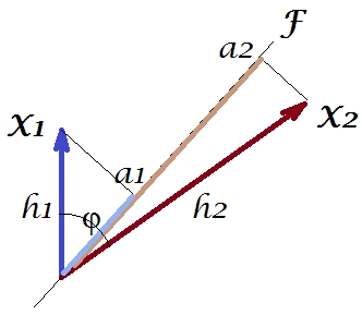
As in a number of my answers on PCA or Factor analysis I will turn to vector representation of variables in subject space. In this instance it is but a loading plot showing variables and their component loadings. So we got $X_1$ and $X_2$ the variables (we had only two in the dataset), $F$ their 1st principal component, with loadings $a_1$ and $a_2$. The angle between the variables is also marked. Variables were centered preliminary, so their squared lengths, $h_1^2$ and $h_2^2$ are their respective variances.

The covariance between $X_1$ and $X_2$ is - it is their scalar product - $h_1 h_2 cos \phi$ (this cosine is the correlation value, by the way). Loadings of PCA, of course, capture the maximum possible of the overall variance $h_1^2+h_2^2$ by $a_1^2+a_2^2$, the component $F$'s variance.
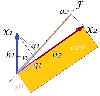
Now, the covariance $h_1 h_2 cos \phi = g_1 h_2$, where $g_1$ is the projection of variable $X_1$ on variable $X_2$ (the projection which is the regression prediction of the first by the second). And so the magnitude of the covariance could be rendered by the area of the rectangle below (with sides $g_1$ and $h_2$).

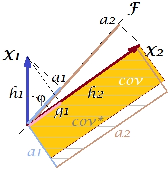
According to the so called "factor theorem" (might know if you read something on factor analysis), covariance(s) between variables should be (closely, if not exactly) reproduced by multiplication of loadings of the extracted latent variable(s) (read). That is, by, $a_1 a_2$, in our particular case (if to recognize the principal component to be our latent variable). That value of the reproduced covariance could be rendered by the area of a rectangle with sides $a_1$ and $a_2$. Let us draw the rectangle, aligned by the previous rectangle, to compare. That rectangle is shown hatched below, and its area is nicknamed cov* (reproduced cov).

It's obvious that the two areas are pretty dissimilar, with cov* being considerably larger in our example. Covariance got overestimated by the loadings of $F$, the 1st principal component. This is contrary to somebody who might expect that PCA, by the 1st component alone of the two possible, will restore the observed value of the covariance.
What could we do with our plot to enchance the reproduction? We can, for example, rotate the $F$ beam clockwise a bit, even until it superposes with $X_2$. When their lines coincide, that means that we forced $X_2$ to be our latent variable. Then loading $a_2$ (projection of $X_2$ on it) will be $h_2$, and loading $a_1$ (projection of $X_1$ on it) will be $g_1$. Then two rectangles are the same one - the one that was labeled cov, and so the covariance is reproduced perfectly. However, $g_1^2 + h_2^2$, the variance explained by the new "latent variable", is smaller than $a_1^2 + a_2^2$, the variance explained by the old latent variable, the 1st principal component (square and stack the sides of each of the two rectangles on the picture, to compare). It appears that we managed to reproduce the covariance, but at expense of explaining the amount of variance. I.e. by selecting another latent axis instead of the first principal component.
Our imagination or guess may suggest (I won't and possibly cannot prove it by math, I'm not a mathematician) that if we release the latent axis from the space defined by $X_1$ and $X_2$, the plane, allowing it to swing a bit towards us, we can find some optimal position of it - call it, say, $F^*$ - whereby the covariance is again reproduced perfectly by the emergent loadings ($a_1^* a_2^*$) while the variance explained ($a_1^{*2} + a_2^{*2}$) will be bigger than $g_1^2 + h_2^2$, albeit not as big as $a_1^2 + a_2^2$ of the principal component $F$.
I believe that this condition is achievable, particularly in that case when the latent axis $F^*$ gets drawn extending out of the plane in such a way as to pull a "hood" of two derived orthogonal planes, one containing the axis and $X_1$ and the other containing the axis and $X_2$. Then this latent axis we'll call the common factor, and our entire "attempt at originality" will be named factor analysis.
Part 2. A reply to @amoeba's "Update 2" in respect to PCA.
@amoeba is correct and relevant to recall Eckart-Young theorem which is fundamental to PCA and its congeneric techniques (PCoA, biplot, correspondence analysis) based on SVD or eigen-decomposition. According to it, $k$ first principal axes of $\bf X$ optimally minimize $\bf ||X-X_k||^2$ - a quantity equal to $\bf tr(X'X)-tr(X_k'X_k)$, - as well as $\bf ||X'X-X_k'X_k||^2$. Here $\bf X_k$ stands for the data as reproduced by the $k$ principal axes. $\bf X_k'X_k$ is known to be equal to $\bf W_k W_k'$, with $\bf W_k$ being the variable loadings of the $k$ components.
Does it mean that minimization $\bf ||X'X-X_k'X_k||^2$ remain true if we consider only off-diagonal portions of both symmetric matrices? Let's inspect it by experimenting.
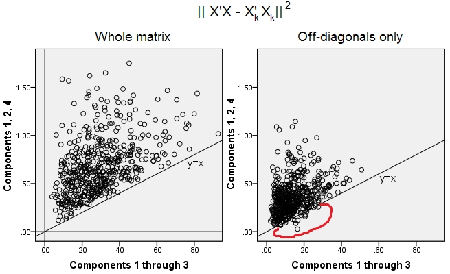
500 random 10x6 matrices $\bf X$ were generated (uniform distribution). For each, after centering its columns, PCA was performed, and two reconstructed data matrices $\bf X_k$ computed: one as reconstructed by components 1 through 3 ($k$ first, as usual in PCA), and the other as reconstructed by components 1, 2, and 4 (that is, component 3 was replaced by a weaker component 4). The reconstruction error $\bf ||X'X-X_k'X_k||^2$ (sum of squared difference = squared Euclidean distance) was then computed for one $\bf X_k$, for the other $\bf X_k$. These two values is a pair to show on a scatterplot.
The reconstruction error was computed each time in two versions: (a) whole matrices $\bf X'X$ and $\bf X_k'X_k$ compared; (b) only off-diagonals of the two matrices compared. Thus, we have two scatterplots, with 500 points each.

We see, that on the "whole matrix" plot all points lie above y=x line. Which means that the reconstruction for the whole scalar-product matrix is always more accurate by "1 through 3 components" than by "1, 2, 4 components". This is in line with Eckart-Young theorem says: first $k$ principal components are the best fitters.
However, when we look at "off-diagonals only" plot we notice a number of points below the y=x line. It appeared that sometimes reconstruction of off-diagonal portions by "1 through 3 components" was worse than by "1, 2, 4 components". Which automatically leads to the conclusion that first $k$ principal components are not regularly the best fitters of off-diagonal scalar products among fitters available in PCA. For example, taking a weaker component instead of a stronger may sometimes improve the reconstruction.
So, even in the domain of PCA itself, senior principal components - who do approximate overall variance, as we know, and even the whole covariance matrix, too, - not necessarily approximate off-diagonal covariances. Better optimization of those is required therefore; and we know that factor analysis is the (or among the) technique that can offer it.
Part 3. A follow-up to @amoeba's "Update 3": Does PCA approach FA as the number of variables grows? Is PCA a valid substitute of FA?
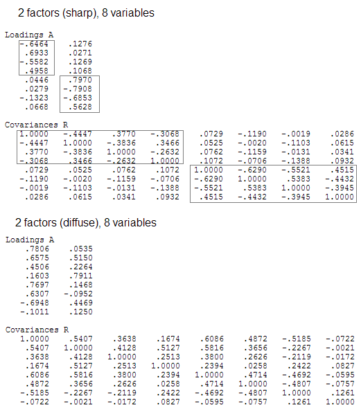
I've conducted a lattice of simulation studies. A few number of population factor structures, loading matrices $\bf A$ were constructed of random numbers and converted to their corresponding population covariance matrices as $\bf R=AA'+ U^2$, with $\bf U^2$ being a diagonal noise (unique variances). These covariance matrices were made with all variances 1, therefore they were equal to their correlation matrices.
Two types of factor structure were designed - sharp and diffuse. Sharp structure is one having clear simple structure: loadings are either "high" of "low", no intermediate; and (in my design) each variable is highly loaded exactly by one factor. Corresponding $\bf R$ is hence noticebly block-like. Diffuse structure does not differentiate between high and low loadings: they can be any random value within a bound; and no pattern within loadings is conceived. Consequently, corresponding $\bf R$ comes smoother. Examples of the population matrices:

The number of factors was either $2$ or $6$. The number of variables was determined by the ratio k = number of variables per factor; k ran values $4,7,10,13,16$ in the study.
For each of the few constructed population $\bf R$, $50$ its random realizations from Wishart distribution (under sample size n=200) were generated. These were sample covariance matrices. Each was factor-analyzed by FA (by principal axis extraction) as well as by PCA. Additionally, each such covariance matrix was converted into corresponding sample correlation matrix that was also factor-analyzed (factored) same ways. Lastly, I also performed factoring of the "parent", population covariance (=correlation) matrix itself. Kaiser-Meyer-Olkin measure of sampling adequacy was always above 0.7.
For data with 2 factors, the analyses extracted 2, and also 1 as well as 3 factors ("underestimation" and "overestimation" of the correct number of factors regimes). For data with 6 factors, the analyses likewise extracted 6, and also 4 as well as 8 factors.
The aim of the study was the covariances/correlations restoration qualities of FA vs PCA. Therefore residuals of off-diagonal elements were obtained. I registered residuals between the reproduced elements and the population matrix elements, as well as residuals between the former and the analyzed sample matrix elements. The residuals of the 1st type were conceptually more interesting.
Results obtained after analyses done on sample covariance and on sample correlation matrices had certain differences, but all the principal findings occured to be similar. Therefore I'm discussing (showing results) only of the "correlations-mode" analyses.
1. Overall off-diagonal fit by PCA vs FA
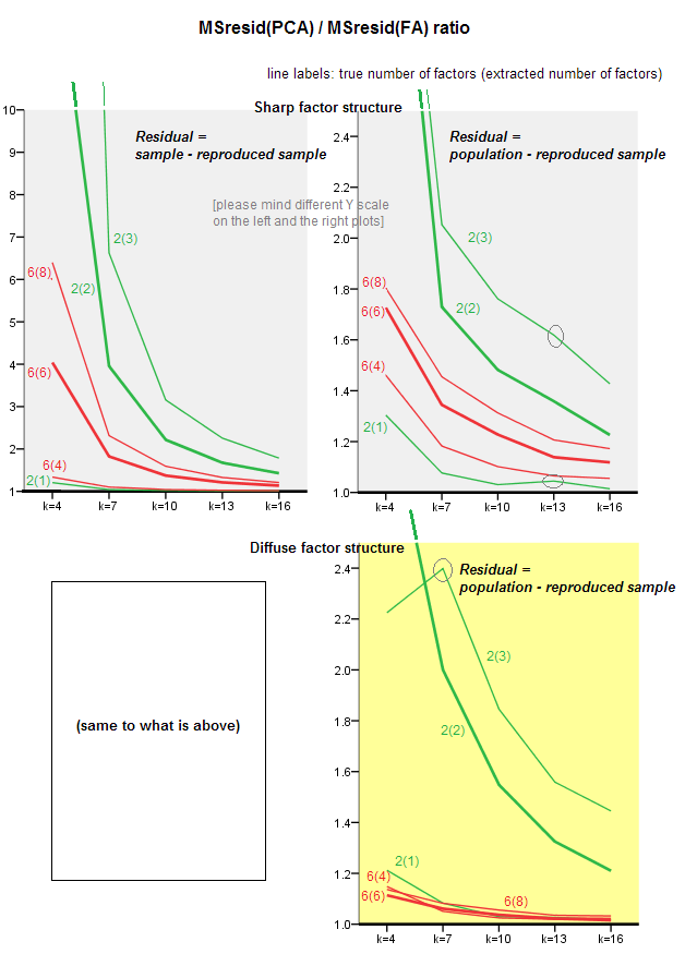
The graphics below plot, against various number of factors and different k, the ratio of the mean squared off-diagonal residual yielded in PCA to the same quantity yielded in FA. This is similar to what @amoeba showed in "Update 3". The lines on the plot represent average tendencies across the 50 simulations (I omit showing st. error bars on them).
(Note: the results are about factoring of random sample correlation matrices, not about factoring the population matrix parental to them: it is silly to compare PCA with FA as to how well they explain a population matrix - FA will always win, and if the correct number of factors is extracted, its residuals will be almost zero, and so the ratio would rush towards infinity.)

Commenting these plots:
- General tendency: as k (number of variables per factor) grows the PCA/FA overall subfit ratio fades towards 1. That is, with more variables PCA approaches FA in explaining off-diagonal correlations/covariances. (Documented by @amoeba in his answer.) Presumably the law approximating the curves is ratio= exp(b0 + b1/k) with b0 close to 0.
- Ratio is greater w.r.t. residuals “sample minus reproduced sample” (left plot) than w.r.t. residuals “population minus reproduced sample” (right plot). That is (trivially), PCA is inferior to FA in fitting the matrix being immediately analyzed. However, lines on the left plot have faster rate of decrease, so by k=16 the ratio is below 2, too, as it is on the right plot.
- With residuals “population minus reproduced sample”, trends are not always convex or even monotonic (the unusual elbows are shown circled). So, as long as speech is about explaining a population matrix of coefficients via factoring a sample, rising the number of variables does not regularly bring PCA closer to FA in its fittinq quality, though the tendency is there.
- Ratio is greater for m=2 factors than for m=6 factors in population (bold red lines are below bold green lines). Which means that with more factors acting in the data PCA sooner catches up with FA. For example, on the right plot k=4 yields ratio about 1.7 for 6 factors, while the same value for 2 factors is reached at k=7.
- Ratio is higher if we extract more factors relative the true number of factors. That is, PCA is only slightly worse a fitter than FA if at extraction we underestimate the number of factors; and it loses more to it if the number of factors is correct or overestimated (compare thin lines with bold lines).
- There is an interesting effect of the sharpness of factor structure which appears only if we consider residuals “population minus reproduced sample”: compare grey and yellow plots on the right. If population factors load variables diffusely, red lines (m=6 factors) sink to the bottom. That is, in diffuse structure (such as loadings of chaotic numbers) PCA (performed on a sample) is only few worse than FA in reconstructing the population correlations- even under small k, provided that the number of factors in the population isn’t very small. This is probably the condition when PCA is most close to FA and is most warranted as its cheeper substitute. Whereas in the presence of sharp factor structure PCA isn’t so optimistic in reconstructing the population correlations (or covariances): it approaches FA only in big k perspective.
2. Element-level fit by PCA vs FA: distribution of residuals
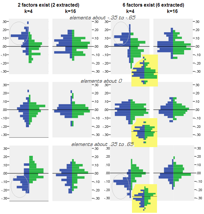
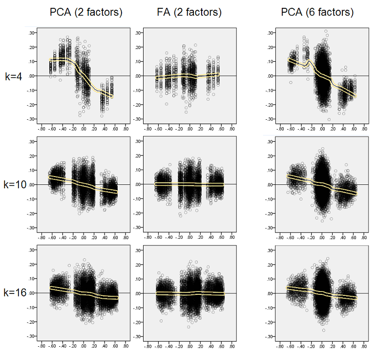
For every simulation experiment where factoring (by PCA or FA) of 50 random sample matrices from the population matrix was performed, distribution of residuals "population correlation minus reproduced (by the factoring) sample's correlation" was obtained for every off-diagonal correlation element. Distributions followed clear patterns, and examples of typical distributions are depicted right below. Results after PCA factoring are blue left sides and results after FA factoring are green right sides.

The principal finding is that
- Pronounced, by absolute magnitude, population correlations are restored by PCA inadequetly: the reproduced values are overestimates by magnitude.
- But the bias vanishes as k (number of variables to number of factors ratio) increases. On the pic, when there is only k=4 variables per factor, PCA's residuals spread in offset from 0. This is seen both when there exist 2 factors and 6 factors. But with k=16 the offset is hardly seen - it almost dissapeared and PCA fit approaches FA fit. No difference in spread (variance) of residuals between PCA and FA is observed.
Similar picture is seen also when the number of factors extracted does not match true number of factors: only variance of residuals somewhat change.
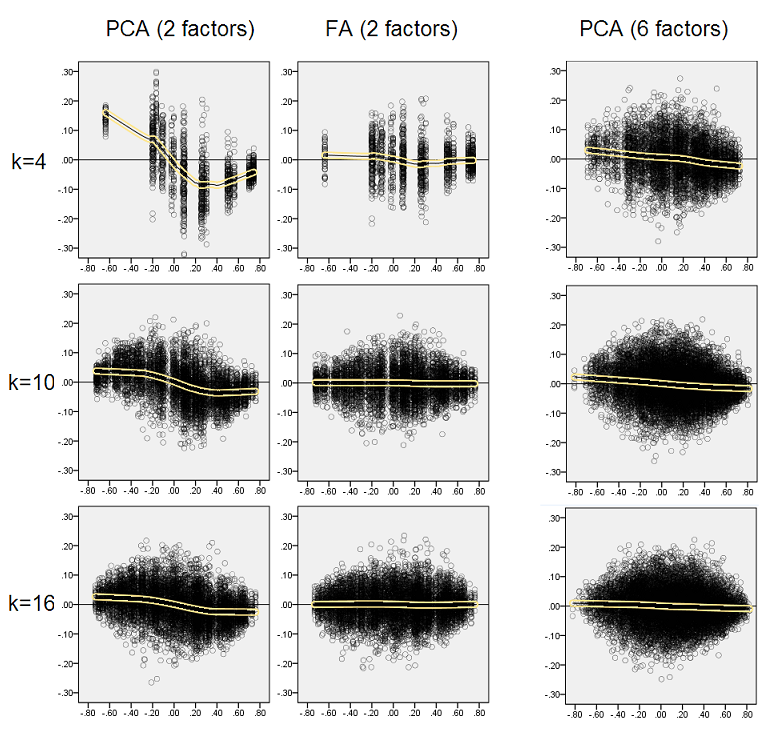
The distributions shown above on grey background pertain to the experiments with sharp (simple) factor structure present in the population. When all the analyses were done in situation of diffuse population factor structure, it was found that the bias of PCA fades away not only with the rise of k, but also with the rise of m (number of factors). Please see the scaled down yellow-background attachments to the column "6 factors, k=4": there is almost no offset from 0 observed for PCA results (the offset is yet present with m=2, that is not shown on the pic).
Thinking that the described findings are important I decided to inspect those residual distributions deeper and plotted the scatterplots of the residuals (Y axis) against the element (population correlation) value (X axis). These scatterplots each combine results of all the many (50) simulations/analyses. LOESS fit line (50% local points to use, Epanechnikov kernel) is highlighted. The first set of plots is for the case of sharp factor structure in the population (the trimodality of correlation values is apparent therefore):

Commenting:
- We clearly see the (described above) reconstuction bias which is
characteristic of PCA as the skew, negative trend loess line: big in
absolute value population correlations are overestimated by PCA of
sample datasets. FA is unbiased (horizontal loess).
- As k grows, PCA's bias diminishes.
- PCA is biased irrespective of how many factors there are in the population: with 6 factors existent (and 6 extracted at analyses) it is similarly defective as with 2 factors existent (2 extracted).
The second set of plots below is for the case of diffuse factor structure in the population:

Again we observe the bias by PCA. However, as opposed to sharp factor structure case, the bias fades as the number of factors increases: with 6 population factors, PCA's loess line is not very far from being horizontal even under k only 4. This is what we've expressed by "yellow histograms" earlier.
One interesting phenomenon on both sets of scatterplots is that loess lines for PCA are S-curved. This curvature shows under other population factor structures (loadings) randomly constructed by me (I checked), although its degree varies and is often weak. If follows from the S-shape then that PCA starts to distort correlations rapidly as they bounce from 0 (especially under small k), but from some value on - around .30 or .40 - it stabilizes. I will not speculate at this time for possible reason of that behavior, althougt I believe the "sinusoid" stems from the triginometric nature of correlation.
3. Fit by PCA vs FA: Conclusions
As the overall fitter of the off-diagonal portion of a correlation/covariance matrix, PCA - when applied to analyze a sample matrix from a population - can be a fairly good substitute for factor analysis. This happens when the ratio number of variables / number of expected factors is big enough. (Geometrical reason for the beneficial effect of the ratio is explained in the bottom Footnote $^1$.) With more factors existent the ratio may be less than with only few factors. The presence of sharp factor structure (simple structure exists in the population) hampers PCA to approach the quality of FA.
The effect of sharp factor structure on the overall fit ability of PCA is apparent only as long as residuals "population minus reproduced sample" are considered. Therefore one can miss to recognize it outside a simulation study setting - in an observational study of a sample we don't have access to these important residuals.
Unlike factor analysis, PCA is a (positively) biased estimator of the magnitude of population correlations (or covariances) that are away from zero. The biasedness of PCA however decreases as the ratio number of variables / number of expected factors grows. The biasedness also decreases as the number of factors in the population grows, but this latter tendency is hampered under a sharp factor structure present.
I would remark that PCA fit bias and the effect of sharp structure on it can be uncovered also in considering residuals "sample minus reproduced sample"; I simply omitted showing such results because they seem not to add new impressions.
My very tentative, broad advice in the end might be to refrain from using PCA instead of FA for typical (i.e. with 10 or less factors expected in the population) factor analytic purposes unless you have some 10+ times more variables than the factors. And the fewer are factors the severer is the necessary ratio. I would further not recommend using PCA in place of FA at all whenever data with well-established, sharp factor structure is analyzed - such as when factor analysis is done to validate the being developed or already launched psychological test or questionnaire with articulated constructs/scales . PCA may be used as a tool of initial, preliminary selection of items for a psychometric instrument.
Limitations of the study. 1) I used only PAF method of factor extraction. 2) The sample size was fixed (200). 3) Normal population was assumed in sampling the sample matrices. 4) For sharp structure, there was modeled equal number of variables per factor. 5) Constructing population factor loadings I borrowed them from roughly uniform (for sharp structure - trimodal, i.e. 3-piece uniform) distribution. 6) There could be oversights in this instant examination, of course, as anywhere.
Footnote $1$. PCA will mimic results of FA and become the equivalent fitter of the correlations when - as said here - error variables of the model, called unique factors, become uncorrelated. FA seeks to make them uncorrelated, but PCA doesn't, they may happen to be uncorrelated in PCA. The major condition when it may occur is when the number of variables per number of common factors (components kept as common factors) is large.
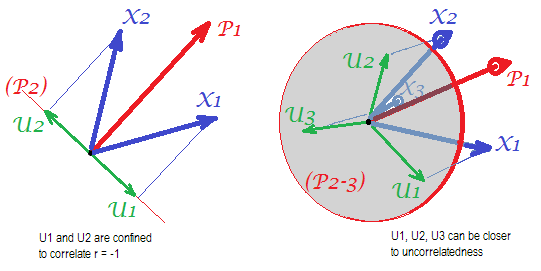
Consider the following pics (if you need first to learn how to understand them, please read this answer):

By the requirement of factor analysis to be able to restore succesfully correlations with few m common factors, unique factors $U$, characterizing statistically unique portions of the p manifest variables $X$, must be uncorrelated. When PCA is used, the p $U$s have to lie in the p-m subspace of the p-space spanned by the $X$s because PCA does not leave the space of the analyzed variables. Thus - see the left pic - with m=1 (principal component $P_1$ is the extracted factor) and p=2 ($X_1$, $X_2$) analyzed, unique factors $U_1$, $U_2$ compulsorily superimpose on the remaining second component (serving as error of the analysis). Consequently they have to be correlated with $r=-1$. (On the pic, correlations equal cosines of angles between vectors.) The required orthogonality is impossible, and the observed correlation between the variables can never be restored (unless the unique factors are zero vectors, a trivial case).
But if you add one more variable ($X_3$), right pic, and extract still one pr. component as the common factor, the three $U$s have to lie in a plane (defined by the remaining two pr. components). Three arrows can span a plane in a way that angles between them are smaller than 180 degrees. There freedom for the angles emerges. As a possible particular case, the angles can be about equal, 120 degrees. That is already not very far from 90 degrees, that is, from uncorrelatedness. This is the situation shown on the pic.
As we add 4th variable, 4 $U$s will be spanning 3d space. With 5, 5 to span 4d, etc. Room for a lot of the angles simultaneously to attain closer to 90 degrees will expand. Which means that the room for PCA to approach FA in its ability to fit off-diagonal triangles of correlation matrix will also expand.
But true FA is usually able to restore the correlations even under small ratio "number of variables / number of factors" because, as explained here (and see 2nd pic there) factor analysis allows all the factor vectors (common factor(s) and unique ones) to deviate from lying in the variables' space. Hence there is the room for the orthogonality of $U$s even with only 2 variables $X$ and one factor.
The more diffuse (the less sharp) is the factor structure - that is, the more unimodal or even is the distribution of the factor loadings, - the closer the above said orthogonality is to become real, realized; the better is PCA executing the role of FA.
The pics above also give obvious clue to why PCA overestimates correlations. On the left pic, for example, $r_{X_1X_2}= a_1a_2 - u_1u_2$, where the $a$s are the projections of the $X$s on $P_1$ (loadings of $P_1$) and the $u$s are the lengths of the $U$s (loadings of $P_2$). But that correlation as reconstructed by $P_1$ alone equals just $a_1a_2$, i.e. bigger than $r_{X_1X_2}$.

