What does AUC stand for and what is it?

Question

Searched high and low and have not been able to find out what AUC, as in related to prediction, stands for or means.

Answer 1

Abbreviations

• AUC = Area Under the Curve.
• AUROC = Area Under the Receiver Operating Characteristic curve.

AUC is used most of the time to mean AUROC, which is a bad practice since as Marc Claesen pointed out AUC is ambiguous (could be any curve) while AUROC is not.

---

Interpreting the AUROC

The AUROC has several equivalent interpretations:

• The expectation that a uniformly drawn random positive is ranked before a uniformly drawn random negative.
• The expected proportion of positives ranked before a uniformly drawn random negative.
• The expected true positive rate if the ranking is split just before a uniformly drawn random negative.
• The expected proportion of negatives ranked after a uniformly drawn random positive.
• The expected false positive rate if the ranking is split just after a uniformly drawn random positive.

Going further: How to derive the probabilistic interpretation of the AUROC?

---

Computing the AUROC

Assume we have a probabilistic, binary classifier such as logistic regression.

Before presenting the ROC curve (= Receiver Operating Characteristic curve), the concept of confusion matrix must be understood. When we make a binary prediction, there can be 4 types of outcomes:

• We predict 0 while the true class is actually 0: this is called a True Negative, i.e. we correctly predict that the class is negative (0). For example, an antivirus did not detect a harmless file as a virus .
• We predict 0 while the true class is actually 1: this is called a False Negative, i.e. we incorrectly predict that the class is negative (0). For example, an antivirus failed to detect a virus.
• We predict 1 while the true class is actually 0: this is called a False Positive, i.e. we incorrectly predict that the class is positive (1). For example, an antivirus considered a harmless file to be a virus.
• We predict 1 while the true class is actually 1: this is called a True Positive, i.e. we correctly predict that the class is positive (1). For example, an antivirus rightfully detected a virus.

To get the confusion matrix, we go over all the predictions made by the model, and count how many times each of those 4 types of outcomes occur:

In this example of a confusion matrix, among the 50 data points that are classified, 45 are correctly classified and the 5 are misclassified.

Since to compare two different models it is often more convenient to have a single metric rather than several ones, we compute two metrics from the confusion matrix, which we will later combine into one:

• True positive rate (TPR), aka. sensitivity, hit rate, and recall, which is defined as $ \frac{TP}{TP+FN}$. Intuitively this metric corresponds to the proportion of positive data points that are correctly considered as positive, with respect to all positive data points. In other words, the higher TPR, the fewer positive data points we will miss.
• False positive rate (FPR), aka. fall-out, which is defined as $ \frac{FP}{FP+TN}$. Intuitively this metric corresponds to the proportion of negative data points that are mistakenly considered as positive, with respect to all negative data points. In other words, the higher FPR, the more negative data points will be missclassified.

To combine the FPR and the TPR into one single metric, we first compute the two former metrics with many different threshold (for example $0.00; 0.01, 0.02, \dots, 1.00$) for the logistic regression, then plot them on a single graph, with the FPR values on the abscissa and the TPR values on the ordinate. The resulting curve is called ROC curve, and the metric we consider is the AUC of this curve, which we call AUROC.

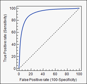
The following figure shows the AUROC graphically:

In this figure, the blue area corresponds to the Area Under the curve of the Receiver Operating Characteristic (AUROC). The dashed line in the diagonal we present the ROC curve of a random predictor: it has an AUROC of 0.5. The random predictor is commonly used as a baseline to see whether the model is useful.

If you want to get some first-hand experience:

• Python: http://scikit-learn.org/stable/auto_examples/model_selection/plot_roc.html
• MATLAB: http://www.mathworks.com/help/stats/perfcurve.html

Answer 2

Although I'm a bit late to the party, but here's my 5 cents. @FranckDernoncourt (+1) already mentioned possible interpretations of AUC ROC, and my favorite one is the first on his list (I use different wording, but it's the same):

the AUC of a classifier is equal to the probability that the classifier will rank a randomly chosen positive example higher than a randomly chosen negative example, i.e. $P\Big(\text{score}(x^+) > \text{score}(x^-)\Big)$

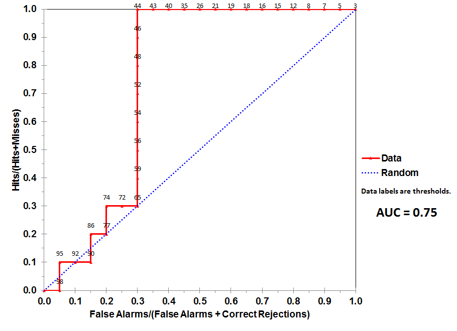
Consider this example (auc=0.68):

Let's try to simulate it: draw random positive and negative examples and then calculate the proportion of cases when positives have greater score than negatives

cls = c('P', 'P', 'N', 'P', 'P', 'P', 'N', 'N', 'P', 'N', 'P',
        'N', 'P', 'N', 'N', 'N', 'P', 'N', 'P', 'N')
score = c(0.9, 0.8, 0.7, 0.6, 0.55, 0.51, 0.49, 0.43, 0.42, 0.39, 0.33, 
          0.31, 0.23, 0.22, 0.19, 0.15, 0.12, 0.11, 0.04, 0.01)

pos = score[cls == 'P']
neg = score[cls == 'N']

set.seed(14)
p = replicate(50000, sample(pos, size=1) > sample(neg, size=1))
mean(p)

And we get 0.67926. Quite close, isn't it?

 

By the way, in R I typically use ROCR package for drawing ROC curves and calculating AUC.

library('ROCR')

pred = prediction(score, cls)
roc = performance(pred, "tpr", "fpr")

plot(roc, lwd=2, colorize=TRUE)
lines(x=c(0, 1), y=c(0, 1), col="black", lwd=1)

auc = performance(pred, "auc")
auc = unlist([email protected])
auc

Answer 3

Important considerations are not included in any of these discussions. The procedures discussed above invite inappropriate thresholding and utilize improper accuracy scoring rules (proportions) that are optimized by choosing the wrong features and giving them the wrong weights.

Dichotomization of continuous predictions flies in the face of optimal decision theory. ROC curves provide no actionable insights. They have become obligatory without researchers examining the benefits. They have a very large ink:information ratio.

Optimum decisions don't consider "positives" and "negatives" but rather the estimated probability of the outcome. The utility/cost/loss function, which plays no role in ROC construction hence the uselessness of ROCs, is used to translate the risk estimate to the optimal (e.g., lowest expected loss) decision.

The goal of a statistical model is often to make a prediction, and the analyst should often stop there because the analyst may not know the loss function. Key components of the prediction to validate unbiasedly (e.g., using the bootstrap) are the predictive discrimination (one semi-good way to measure this is the concordance probability which happens to equal the area under the ROC but can be more easily understood if you don't draw the ROC) and the calibration curve. Calibration validation is really, really necessary if you are using predictions on an absolute scale.

See the Information Loss chapter in Biostatistics for Biomedical Research and other chapters for more information.

Answer 4

The answers in this forum are great and I come back here often for reference. However, one thing was always missing. From @Frank's answer, we see the interpretation of AUC as the probability that a positive sample will have a higher score than the negative sample. At the same time, the way to calculate it is to plot out the TPR and FPR as the threshold, $\tau$ is changed and calculate the area under that curve. But, why is this area under the curve the same as this probability? @Alexy showed through simulation that they're close, but can we derive this relationship mathematically? Let's assume the following:

1. $A$ is the distribution of scores the model produces for data points that are actually in the positive class.
2. $B$ is the distribution of scores the model produces for data points that are actually in the negative class (we want this to be to the left of $A$).
3. $\tau$ is the cutoff threshold. If a data point get's a score greater than this, it's predicted as belonging to the positive class. Otherwise, it's predicted to be in the negative class.

Note that the TPR (recall) is given by: $P(A>\tau)$ and the FPR (fallout) is given be: $P(B>\tau)$.

Now, we plot the TPR on the y-axis and FPR on the x-axis, draw the curve for various $\tau$ and calculate the area under this curve ($AUC$).

We get:

$$AUC = \int_0^1 TPR(x)dx = \int_0^1 P(A>\tau(x))dx$$ where $x$ is the FPR. Now, one way to calculate this integral is to consider $x$ as belonging to a uniform distribution. In that case, it simply becomes the expectation of the $TPR$ since the PDF of the uniform is 1.

$$AUC = E_x[P(A>\tau(x))] \tag{1}$$ if we consider $x \sim U[0,1)$ .

Now, $x$ here was just the $FPR$

$$x=FPR = P(B>\tau(x))$$ Since we considered $x$ to be from a uniform distribution,

$$P(B>\tau(x)) \sim U$$ $$=> P(B<\tau(x)) \sim (1-U) \sim U$$ \begin{equation}=> F_B(\tau(x)) \sim U \tag{2}\end{equation}

But we know from the inverse transform law that for any random variable $X$, if $F_X(Y) \sim U$ then $Y \sim X$. This follows since taking any random variable and applying its own CDF to it leads to the uniform.

$$F_X(X) = P(F_X(x)<X) =P(X<F_X^{-1}(X))=F_XF_X^{-1}(X)=X$$ and this only holds for uniform.

Using this fact in equation (2) gives us: $$\tau(x) \sim B$$

Substituting this into equation (1) we get:

$$AUC=E_x(P(A>B))=P(A>B)$$

In other words, the area under the curve is the probability that a random positive sample will have a higher score than a random negative sample.

Answer 5

AUC is an abbrevation for area under the curve. It is used in classification analysis in order to determine which of the used models predicts the classes best.

An example of its application are ROC curves. Here, the true positive rates are plotted against false positive rates. An example is below. The closer AUC for a model comes to 1, the better it is. So models with higher AUCs are preferred over those with lower AUCs.

Please note, there are also other methods than ROC curves but they are also related to the true positive and false positive rates, e. g. precision-recall, F1-Score or Lorenz curves.

                                           

Answer 6

Very late to respond but after learning from multiple sources I've been able to form my own understanding of the AUC. This response is mainly heuristic in nature and not meant to be rigorous

Let's say we have M positive samples and N negative samples and some "score funcion $s(x)$" that assigns a value to sample $x$. For a threshold $T$ if $s(x)>T$ it's "positive" else it is "negative".

Let's select a negative sample $x_n$ randomly with equal probability $\frac{1}{N}$. If the threshold $T$ is placed at $s(x_n)$ then the true positive rate $TP(T)$ at threshold $T$ is the probability of ranking a randomly selected positive sample $x_p$ above $x_n$. In other words, this occurrence is $P(X_p>X_n|X_n=x_n)=TP(T)$ for $T=s(x_n)$. If both these events occur ($X_n=x_n$ and $x_p>x_n$) then the probability of this occurrence is $P(X_p>X_n|X_n=x_n)P(X_n=x_n)=P(X_p>X_n\cap X_n=x_n)$. From law of total probability, the sum of all these values over all possible values of $x_n$ gives $P(X_p>X_n)$

$$P(X_p>X_n)=\sum_{i=1}^N{P(X_p>X_n\cap X_n=x_i)}$$

$$= \sum_{i=1}^N{P(X_p>X_n|X_n=x_i)P(X_n=x_i)}$$

$$=\sum_{i=1}^N{TP(s(x_i))\frac{1}{N}} $$

In the ROC curve, each time the curve shifts left or right, it means it has "jumped over" a negative sample. When it moves up or down, it means it has "jumped over" a positive sample, which precisely gives the staircase nature of the curve. For the sum above, in the limit as the number of samples becomes infinite we take this sum at all possible values for the false positive rate $FP(T)$ over all these jumps and we get

$$\int_0^1{TP(FP^{-1}(x))dx} $$ for all possible values of threshold $FP^{-1}(x)$ which, using law of total probability, gives the total $$P(X_p>X_n)$$ which is seen to be the area under the ROC curve, AUC

Answer 7

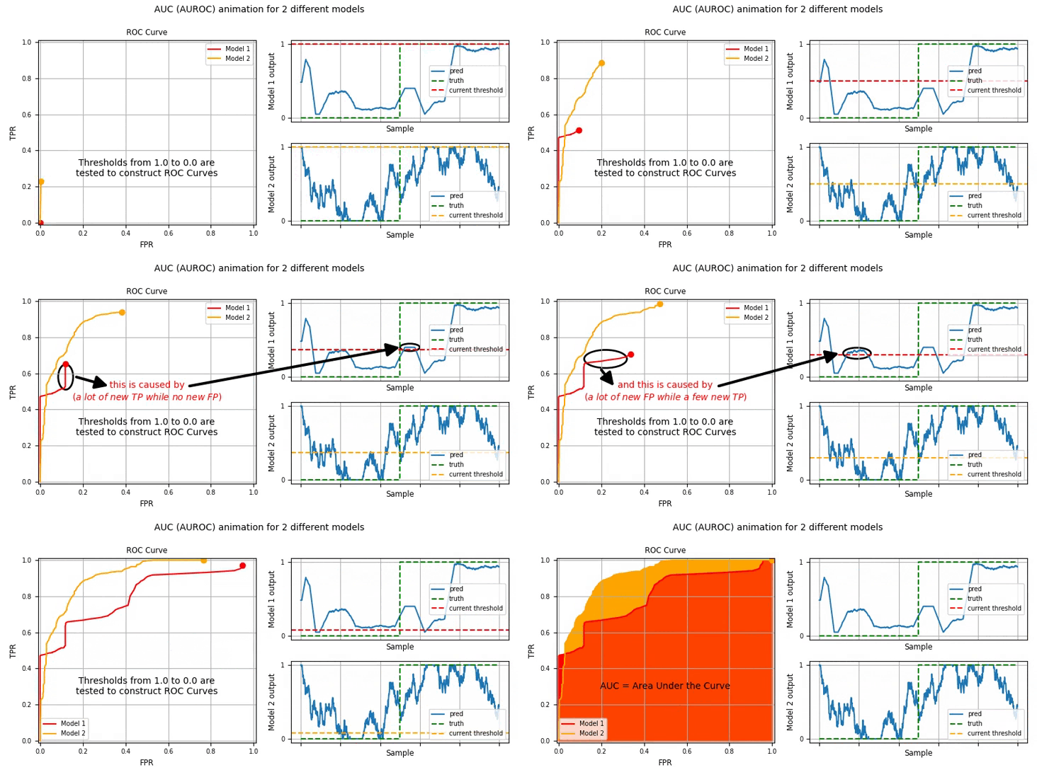
I just wanted to share an animation about the construction of the ROC Curve and so the AUC. One sees clearly that each point of the ROC Curve comes from a different threshold used to classify the output of a binary classifier. The threshold defines which samples are predicted as 1 and which ones as 0. True Positive and False Positive rates are then computed. At every threshold corresponds a point on the ROC Curve.

Note: The animation might be more relevant for people working on time-series, but could also help to understand the AUC construction in other cases as a Sample, the input of the binary classifier, could be anything (image, time-serie window, input features,...)