We can take a tip from the literature on outlier detection. In effect, this dataset can be summarized as a sequence of counts of the 35 benefits. The null hypothesis is that the counts were generated by a process in which individuals chose benefits completely at random and independently of one another. The alternative you want to be able to detect is that some previously unknown number $r \ge 0$ of the counts are chosen more frequently than the rest.
Good tests for this situation (of an unknown number of high outliers) often rely on gaps, and that's precisely the statistic highlighted in the clarification to the question: "The top three benefits were at least 10 votes clear of the fourth most popular." But, to be thoroughly honest in our analysis, let's look at the problem as if we did not know the results yet.
A priori, then, it looks like identifying an unusually large gap among the highest counts might do a good job of separating counts that are too high to be explained by chance. But another alternative may also be of interest: it could be that each benefit (as indexed, say, by $1 \le i \le 35$) is chosen with probability $p_i$ and that there is a slight but important amount of variation among the $p_i$. This could lead to a graduated series of elevated counts: e.g., one benefit might be chosen $19$ times, another $18$ times, another $17$ times, ..., etc, thereby exhibiting no unusual gaps in the counts. It would be good to detect this situation, too.
I am thereby led to propose a two-criterion test based on a pair of statistics: the highest count and the largest gap among the highest half of all the counts (because we're not interested in any low outliers).
The crucial thing is to establish the joint distribution of these statistics under the null hypothesis (to wit, $p_1 = p_2 = \cdots = p_{35}$). That we can readily do with simulation. The following results are each based on 1,000,000 independent replications of the experiment; each set of results is derived from a separate set of such replications.
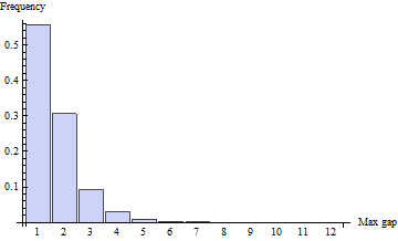
Null distribution of the largest gaps

The estimated complementary cumulative distribution function (good to 3-5 decimal places based on this simulation) is
Max gap   p
1         1.000
2         0.442
3         0.136
4         0.0434
5         0.0135
6         0.0039
7         0.00011
8         0.00003
9        <0.00001
Thus, if you wished to use the max gap test to identify high outliers at the $\alpha=5\%$ level, you would read down this chart until $p$ first fell below $5\%$, finding the critical value of $4$. According to this test, if the largest gap among the top half of the counts (sorted from smallest to largest) were $4$ or greater, you would conclude that some benefits are selected significantly more frequently than others, and those would be all those with counts occurring above the lowest gap of $4$ or more occurring among the top half of all counts.
For example, one trial resulted in the following:
- Three benefits were each selected by 3 people
- Five benefits were each selected by 4 people
- Four ... 5
- Eleven ... 6
- Three ... 7
- Seven ... 8
- One ... 9
- One benefit was selected by 14 people.
We could equally well say that the ordered set of counts is
14, 9, 8, 8, 8, 8, 8, 8, 8, 7, ..., 4, 3, 3, 3.
(As a check, $3*3 + 5*4 + 4*5 + 11*6 + 3*7 + 7*8 + 1*9 + 1*14 = 215$ accounts for all $5*43$ choices.) In this trial, the upper half of the counts comprise those $6$ or greater. The nonzero gaps, starting at $6$, are $7-6=1$, $8-7=1$, $9-8=1$, and $14-9=5$. The last is the largest gap and only the count of $14$ exceeds it. We conclude (a) there is at least one benefit chosen significantly more than the rest and (b) it consists of just the one benefit that was chosen by $14$ people.
In another case, two benefits were each selected by $9$ people, one benefit by $14$ people, and one benefit by $15$ people. Here the maximum gap was $k=14-9=5$ and two benefits are identified as chosen significantly more than the rest.
In yet another case, the ordered set of counts was
21, 15, 15, 14, 14, 14, 10, 10, 9, ... .
The max gap is $21-15=6$. However, there's another gap of at least $4$ among the highest counts: $14-10=4$. Therefore, the six highest counts would be considered elevated (to wit, $21, 15, 15, 14, 14, 14$) at the $5\%$ level.
Conditional distribution of the highest frequencies
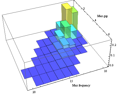
In case the maximum gap test fails to detect any significantly high choice, it is still possible that many choices may have been selected more frequently than on average. Our supplemental test for this situation looks at the highest frequency. To investigate this, we need to evaluate the joint distribution of the maximum gap and the highest frequency when the maximum gap is less than the critical value of the maximum gap test.
Here is a plot of the joint distribution under the null hypothesis (at least where the probabilities are visibly greater than zero). For a better view, it is shown with axes reversed: larger values of both statistics occur near the front.

As we have seen, in many applications the critical value will be either $4$ (for $\alpha \approx 5\%$) or $5$ (for $\alpha = 1.35\%$) or possibly $6$ (for $\alpha \approx 0.4\%$). We would then only need to inspect the maximum frequency when the maximum gap is less than or equal to $3$ (or $4$ or $5$, respectively). Here is a detail of the joint distribution plot for this region:

Suppose, for example, we still want to conduct a test at the $\alpha=5\%$ level. We saw above that this indicates a critical threshold of $4$ for the max gap test. The actual level achieved by this test is $4.34\%$. This leaves a little room to screen by maximum frequency. The simulation shows that when the maximum gap is less than $4$, we can also include any dataset whose maximum frequency is $15$ or larger within the critical region. When the null hypothesis is true, this joint test statistic lies in the critical region $4.73\%$ of the time: comfortably close to the desired $5\%$ level. (If we were more aggressively to include a maximum frequency of $14$ within the critical region, $\alpha$ would jump to about $7.7\%$, too far above the targeted value of $5\%$.)
For example, suppose the highest counts are $15, 14, 12, 10, 8, 8,$ etc, with a maximum gap of $14-12=2$. This would not be identified as significant with the max gap test (at $\alpha \approx 5\%$), but the maximum value of $15$ is evidence of some tendency to select at least one (but some unknown) number of benefits more often.
Other good combinations for critical values of (max gap, max frequency) are:
(4, 15): 4.7%
(5, 16): 1.5%   (5, 15): 2.4%
(6, 17): 0.4%   (6, 16): 0.7%
(7, 18): 0.1%   (7, 17): 0.2%
The second instance in each row is more sensitive to slight differences in the $p_i$ while the first instance primarily tests for identifiable high outliers, which is probably what is most desirable here.
Obviously in any similar situation where these parameters (43, 5, 35) are different, the simulations would have to be re-run accordingly. Simulations are needed, by the way, because these parameters are small enough that neither a Poisson approximation nor approximating by a collection of iid Binomials is sufficiently accurate for calculations. Once 5*35 = 215 gets larger and 43 * 5/35 = 6 gets smaller, these approximations can fruitfully replace simulations.
Now let's analyze the data. Reportedly there is a gap of $10$ between the three highest counts and the rest. This identifies the three highest counts as significantly elevated. It's possible that additional gaps of $4$ or greater occur. For instance, the ordered set of counts might be
28, 28, 25, 15, 14, 10, ... .
In this case, if we were testing at the $5\%$ level, we would also identify the two benefits chosen by $15$ and $14$ people as being significantly elevated compared to the rest, because their counts both lie above a gap of $14-10=4$, giving five elevated benefits in toto. If we were testing at the $1\%$ level these two benefits would not be significant, leaving just three elevated benefits. If we were testing at the $2.5\%$ level with critical values of $(5,15)$ we would still only identify three significant benefits: the max frequency test is used only when the max gap is less than its critical value (of $5$).
A note about implementation
The calculations and illustrations presented here were done in Mathematica (8.0). Its language makes a good pseudocode no matter what platform is intended to be used in the end.
The core function, trial, simulates a single experiment:
trial[respondents_, votes_, choices_] :=
  Sort[Rest[BinCounts[Flatten[Table[
       RandomSample[Range[choices], votes], {i, 1, respondents}]], {0, choices+1, 1}]]]
Each "respondent" takes a random sample of votes from the set 1..choices. The results are combined (Flatten) and tallied in integer-width bins (Rest[BinCounts..]) from 1 through choices. The counts are sorted for later analysis. For example, one call to trial[43,5,35] resulted in the array (2, 3, 3, 4, 4, 4, 4, 4, 4, 5, 5, 5, 5, 5, 5, 5, 6, 6, 7, 7, 7, 7, 7, 7, 8, 8, 8, 8, 8, 8, 9, 9, 9, 9, 10), indicating that one choice was selected by two respondents, two other choices were selected by three respondents, etc.
The maximum gap above the median for any such trial t is computed as
maxGap[t_] := Max[Differences[Take[t, Floor[-(Length[t] + 1)/2]]]]
It's just the largest difference among the last (35+1)/2 = 18 elements in t.
A Monte-Carlo simulation of the max gap statistic can then be generated as
data = ParallelTable[maxGap[trial[43, 5, 35]], {i, 1, nTrials=1000000}];
The first illustration, Null Distribution of the Largest Gaps, was created in this way by making a histogram of the gap frequencies:
gapFreq = Sort[Tally[data], First[#1] <= First[#2] &];
BarChart[Last[Transpose[gapFreq]]/nTrials,
 ChartLabels -> First[Transpose[gapFreq]],
 AxesLabel -> {"Max gap", "Frequency"}]
The rest of the analysis similarly computes and displays properties of the simulated data.


