How is Naive Bayes a Linear Classifier?

Question

I've seen the other thread here but I don't think the answer satisfied the actual question. What I have continually read is that Naive Bayes is a linear classifier (ex: here) (such that it draws a linear decision boundary) using the log odds demonstration.

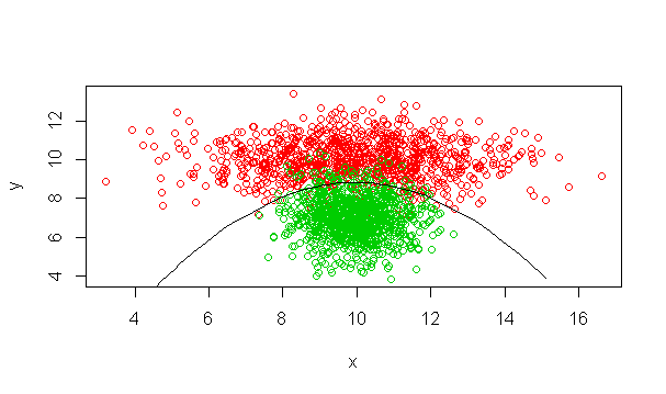
However, I simulated two Gaussian clouds and fitted a decision boundary and got the results as such (library e1071 in r, using naiveBayes())

As we can see, the decision boundary is non-linear. Is it trying to say that the parameters (conditional probabilities) are a linear combination in the log space rather than saying the classifier itself separates data linearly?

Answer 1

In general the naive Bayes classifier is not linear, but if the likelihood factors $p(x_i \mid c)$ are from exponential families, the naive Bayes classifier corresponds to a linear classifier in a particular feature space. Here is how to see this.

You can write any naive Bayes classifier as*

$$p(c = 1 \mid \mathbf{x}) = \sigma\left( \sum_i \log \frac{p(x_i \mid c = 1)}{p(x_i \mid c = 0)} + \log \frac{p(c = 1)}{p(c = 0)} \right),$$

where $\sigma$ is the logistic function. If $p(x_i \mid c)$ is from an exponential family, we can write it as

$$p(x_i \mid c) = h_i(x_i)\exp\left(\mathbf{u}_{ic}^\top \phi_i(x_i) - A_i(\mathbf{u}_{ic})\right),$$

and hence

$$p(c = 1 \mid \mathbf{x}) = \sigma\left( \sum_i \mathbf{w}_i^\top \phi_i(x_i) + b \right),$$

where

\begin{align} \mathbf{w}_i &= \mathbf{u}_{i1} - \mathbf{u}_{i0}, \\ b &= \log \frac{p(c = 1)}{p(c = 0)} - \sum_i \left( A_i(\mathbf{u}_{i1}) - A_i(\mathbf{u}_{i0}) \right). \end{align}

Note that this is similar to logistic regression – a linear classifier – in the feature space defined by the $\phi_i$. For more than two classes, we analogously get multinomial logistic (or softmax) regression.

If $p(x_i \mid c)$ is Gaussian, then $\phi_i(x_i) = (x_i, x_i^2)$ and we should have \begin{align} w_{i1} &= \sigma_1^{-2}\mu_1 - \sigma_0^{-2}\mu_0, \\ w_{i2} &= 2\sigma_0^{-2} - 2\sigma_1^{-2}, \\ b_i &= \log \sigma_0 - \log \sigma_1, \end{align}

assuming $p(c = 1) = p(c = 0) = \frac{1}{2}$.

---

*Here is how to derive this result:

\begin{align} p(c = 1 \mid \mathbf{x}) &= \frac{p(\mathbf{x} \mid c = 1) p(c = 1)}{p(\mathbf{x} \mid c = 1) p(c = 1) + p(\mathbf{x} \mid c = 0) p(c = 0)} \\ &= \frac{1}{1 + \frac{p(\mathbf{x} \mid c = 0) p(c = 0)}{p(\mathbf{x} \mid c = 1) p(c = 1)}} \\ &= \frac{1}{1 + \exp\left( -\log\frac{p(\mathbf{x} \mid c = 1) p(c = 1)}{p(\mathbf{x} \mid c = 0) p(c = 0)} \right)} \\ &= \sigma\left( \sum_i \log \frac{p(x_i \mid c = 1)}{p(x_i \mid c = 0)} + \log \frac{p(c = 1)}{p(c = 0)} \right) \end{align}

Answer 2

It is linear only if the class conditional variance matrices are the same for both classes. To see this write down the ration of the log posteriors and you'll only get a linear function out of it if the corresponding variances are the same. Otherwise it is quadratic.

Answer 3

I'd like add one additional point: the reason for some of the confusion rests on what it means to be performing "Naive Bayes classification".

Under the broad topic of "Gaussian Discriminant Analysis (GDA)" there are several techniques: QDA, LDA, GNB, and DLDA (quadratic DA, linear DA, gaussian naive bayes, diagonal LDA). [UPDATED] LDA and DLDA should be linear in the space of the given predictors. (See, e.g., Murphy, 4.2, pg. 101 for DA and pg. 82 for NB. Note: GNB is not necessarily linear. Discrete NB (which uses a multinomial distribution under the hood) is linear. You can also check out Duda, Hart & Stork section 2.6). QDA is quadratic as other answers have pointed out (and which I think is what is happening in your graphic - see below).

These techniques form a lattice with a nice set of constraints on the "class-wise covariance matrices" $\Sigma_c$:

• QDA: $\Sigma_c$ arbitrary: arbitrary ftr. cov. matrix per class
• LDA: $\Sigma_c = \Sigma$: shared cov. matrix (over classes)
• GNB: $\Sigma_c = {diag}_c$: class wise diagonal cov. matrices (the assumption of ind. in the model $\rightarrow$ diagonal cov. matrix)
• DLDA: $\Sigma_c = diag$: shared & diagonal cov. matrix

While the docs for e1071 claim that it is assuming class-conditional independence (i.e., GNB), I'm suspicious that it is actually doing QDA. Some people conflate "naive Bayes" (making independence assumptions) with "simple Bayesian classification rule". All of the GDA methods are derived from the later; but only GNB and DLDA use the former.

A big warning, I haven't read the e1071 source code to confirm what it is doing.