Intuitive explanation for density of transformed variable?

Question

Suppose $X$ is a random variable with pdf $f_X(x)$. Then the random variable $Y=X^2$ has the pdf

$$f_Y(y)=\begin{cases}\frac{1}{2\sqrt{y}}\left(f_X(\sqrt{y})+f_X(-\sqrt{y})\right) & y \ge 0 \\ 0 & y \lt 0\end{cases}$$

I understand the calculus behind this. But I'm trying to think of a way to explain it to someone who doesn't know calculus. In particular, I'm trying to explain why the factor $\frac{1}{\sqrt{y}}$ appears out front. I'll take a stab at it:

Suppose $X$ has a Gaussian distribution. Almost all the weight of its pdf is between the values, say, $-3$ and $3.$ But that maps to 0 to 9 for $Y$. So, the heavy weight in the pdf for $X$ has been extended across a wider range of values in the transformation to $Y$. Thus, for $f_Y(y)$ to be a true pdf the extra heavy weight must be downweighted by the multiplicative factor $\frac{1}{\sqrt{y}}$

How does that sound?

If anyone can provide a better explanation of their own or link to one in a document or textbook I'd greatly appreciate it. I find this variable transformation example in several intro mathematical probability/stats books. But I never find an intuitive explanation with it :(

Answer 1

PDFs are heights but they are used to represent probability by means of area. It therefore helps to express a PDF in a way that reminds us that area equals height times base.

Initially the height at any value $x$ is given by the PDF $f_X(x)$. The base is the infinitesimal segment $dx$, whence the distribution (that is, the probability measure as opposed to the distribution function) is really the differential form, or "probability element,"

$$\operatorname{PE}_X(x) = f_X(x) \, dx.$$

This, rather than the PDF, is the object you want to work with both conceptually and practically, because it explicitly includes all the elements needed to express a probability.

When we re-express $x$ in terms of $y = x^2$, the base segments $dx$ get stretched (or squeezed): by squaring both ends of the interval from $x$ to $x + dx$ we see that the base of the $y$ area must be an interval of length

$$dy = (x + dx)^2 - x^2 = 2 x \, dx + (dx)^2.$$

Because the product of two infinitesimals is negligible compared to the infinitesimals themselves, we conclude

$$dy = 2 x \, dx, \text{ whence }dx = \frac{dy}{2x} = \frac{dy}{2\sqrt{y}}.$$

Having established this, the calculation is trivial because we just plug in the new height and the new width:

$$\operatorname{PE}_X(x) = f_X(x) \, dx = f_X(\sqrt{y}) \frac{dy}{2\sqrt{y}} = \operatorname{PE}_Y(y).$$

Because the base, in terms of $y$, is $dy$, whatever multiplies it must be the height, which we can read directly off the middle term as

$$\frac{1}{2\sqrt{y}}f_X(\sqrt{y}) = f_Y(y).$$

This equation $\operatorname{PE}_X(x) = \operatorname{PE}_Y(y)$ is effectively a conservation of area (=probability) law.

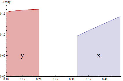
This graphic accurately shows narrow (almost infinitesimal) pieces of two PDFs related by $y=x^2$. Probabilities are represented by the shaded areas. Due to the squeezing of the interval $[0.32, 0.45]$ via squaring, the height of the red region ($y$, at the left) has to be proportionally expanded to match the area of the blue region ($x$, at the right).

Answer 2

How about, if I manufacture objects that are always square and I know the distribution of the side lengths of the squares; what can I say about the distribution of the areas of the squares?

In particular, if I know the distribution of a random variable $X$, what can I say about $Y = X^{2}$? One thing that you can say is

$$\eqalign{ F_{Y} (c) & = & P( Y \le c ) \\ & = & P( X^{2} \le c ) \\ & = & P ( - \sqrt{c} \le X \le \sqrt{c}) \\ & = & F_{X}( \sqrt{c} ) - F_{X}( - \sqrt{c} ). \\ }$$

So a relationship is established between the CDF of $Y$ and CDF of $X$; what is the relationship between their PDFs? We need calculus for that. Taking the derivatives of both sides gives you the results you wanted.

Answer 3

Imagine we have a population and $Y$ is a summary of that population. Then $P(Y \in (y, y + \Delta y))$ is counting the proportion of individuals that have variable $Y$ in the range $(y, y + \Delta y)$. You can consider this as a "bin" of size $\Delta y$ and we are counting how many individuals are inside that bin.

Now let us re-express those individuals in terms of another variable, $X$. Given that we know that $Y$ and $X$ are related as $Y = X^2$, the event $Y\in (y, y + \Delta y)$ is the same as the event $X^2 \in (x^2, (x + \Delta x)^2)$ which is the same as the event $ X \in (|x|, |x| + \Delta x)~ \text{or}~ X \in (- |x| -\Delta x, -|x| )$. Thus, the individuals that are in the bin $(y, y + \Delta y)$ must also be in the bins $(|x|, |x| + \Delta x)$ and $ (- |x| -\Delta x, -|x| )$. In other words, those bins must have the same proportion of individuals,

\begin{align} P(Y \in (y, y + \Delta y)) &=P\left( X \in (|x|, |x| + \Delta x) \right) + P\left( X \in (- |x| -\Delta x, -|x| )\right) \end{align}

Ok, now let's get to the density. First, we need to define what a probability density is. As the name suggests, it is the proportion of individuals per area. That is, we count the share of individuals on that bin and divide by the size of the bin. Since we have established that the proportions of people are the same here, but the size of the bins have changed, we conclude the density will be different. But different by how much?

As we said, the probability density is the proportion of people in the bin divided by the size of the bin, thus the density of $Y$ is given by $f_Y(y):=\frac{P(Y \in (y, y + \Delta y))}{\Delta y}$. Analogously, the probability density of $X$ is given by $f_X(x):=\frac{P(X \in (x, x + \Delta x))}{\Delta x}$.

From our previous result that the population in each bin is the same we then have that,

\begin{align} f_Y(y):=\frac{P(Y \in (y, y + \Delta y))}{\Delta y} &= \frac{P\left( X \in (|x|, |x| + \Delta x) \right) + P\left( X \in (- |x| - \Delta x, -|x| )\right)}{\Delta y} \\ &= \frac{f_X(|x|)\Delta x + f_{X}(-|x|)\Delta x}{\Delta y}\\ &= \frac{\Delta x}{\Delta y} \left(f_X(|x|) + f_{X}(-|x|) \right)\\ &= \frac{\Delta x}{\Delta y} \left(f_X(\sqrt{y}) + f_{X}(-\sqrt{y}) \right) \end{align}

That is, the density $f_X(\sqrt{y}) + f_{X}(-\sqrt{y})$ changes by the factor $\frac{\Delta x}{\Delta y}$, which is the relative size of stretching or squeezing the bin size. In our case, since $y = x^2$ we have that $y + \Delta y = (x + \Delta x )^2 = x^2 + 2x \Delta x + \Delta x^2$. If $\Delta x$ is tiny enough we can ignore $\Delta x ^2$, which implies $\Delta y = 2x \Delta x$ and $\frac{\Delta x}{\Delta y} = \frac{1}{2x} = \frac{1}{2 \sqrt{y}}$, and that is why the factor $\frac{1}{2 \sqrt{y}}$ shows up in the transformation.