Generate a random variable with a defined correlation to an existing variable(s)

Question

For a simulation study I have to generate random variables that show a predefined (population) correlation to an existing variable $Y$.

I looked into the R packages copula and CDVine which can produce random multivariate distributions with a given dependency structure. It is, however, not possible to fix one of the resulting variables to an existing variable.

Any ideas and links to existing functions are appreciated!

 

Conclusion: Two valid answers came up, with different solutions:

1. An R script by caracal, which calculates a random variable with an exact (sample) correlation to a predefined variable
2. An R function I found myself, which calculates a random variable with a defined population correlation to a predefined variable

---

[@ttnphns' addition: I took the liberty to expand the question title from single fixed variable case to arbitrary number of fixed variables; i.e. how to generate a variable having predefined corretation(s) with some fixed, existing variable(s)]

Answer 1

Here's another one: for vectors with mean 0, their correlation equals the cosine of their angle. So one way to find a vector $x$ with exactly the desired correlation $r$, corresponding to an angle $\theta$:

1. get fixed vector $x_1$ and a random vector $x_2$
2. center both vectors (mean 0), giving vectors $\dot{x}_{1}$, $\dot{x}_{2}$
3. make $\dot{x}_{2}$ orthogonal to $\dot{x}_{1}$ (projection onto orthogonal subspace), giving $\dot{x}_{2}^{\perp}$
4. scale $\dot{x}_{1}$ and $\dot{x}_{2}^{\perp}$ to length 1, giving $\bar{x}_{1}$ and $\bar{x}_{2}^{\perp}$
5. $\bar{x}_{2}^{\perp} + (1/\tan(\theta)) \cdot \bar{x}_{1}$ is the vector whose angle to $\bar{x}_{1}$ is $\theta$, and whose correlation with $\bar{x}_{1}$ thus is $r$. This is also the correlation to $x_1$ since linear transformations leave the correlation unchanged.

Here is the code:

n     <- 20                    # length of vector
rho   <- 0.6                   # desired correlation = cos(angle)
theta <- acos(rho)             # corresponding angle
x1    <- rnorm(n, 1, 1)        # fixed given data
x2    <- rnorm(n, 2, 0.5)      # new random data
X     <- cbind(x1, x2)         # matrix
Xctr  <- scale(X, center=TRUE, scale=FALSE)   # centered columns (mean 0)

Id   <- diag(n)                               # identity matrix
Q    <- qr.Q(qr(Xctr[ , 1, drop=FALSE]))      # QR-decomposition, just matrix Q
P    <- tcrossprod(Q)          # = Q Q'       # projection onto space defined by x1
x2o  <- (Id-P) %*% Xctr[ , 2]                 # x2ctr made orthogonal to x1ctr
Xc2  <- cbind(Xctr[ , 1], x2o)                # bind to matrix
Y    <- Xc2 %*% diag(1/sqrt(colSums(Xc2^2)))  # scale columns to length 1

x <- Y[ , 2] + (1 / tan(theta)) * Y[ , 1]     # final new vector
cor(x1, x)                                    # check correlation = rho

For the orthogonal projection $P$, I used the $QR$-decomposition to improve numerical stability, since then simply $P = Q Q'$.

Answer 2

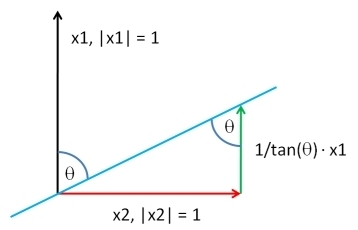
I will describe the most general possible solution. Solving the problem in this generality allows us to achieve a remarkably compact software implementation: just two short lines of R code suffice. At the end is a generalization to multiple $Y$ vectors, with working code.

Pick a vector $X$, of the same length as $Y$, according to any distribution you like. Let $Y^\perp$ be the residuals of the least squares regression of $X$ against $Y$: this removes the $Y$ component from $X,$ producing a vector orthogonal to $Y.$ By adding back a suitable multiple of $Y$ to $Y^\perp$, we may produce a vector having any desired correlation $\rho$ with $Y$ (except $\rho=\pm 1$, but then $\pm Y$ works). Up to an arbitrary additive constant and positive multiplicative constant--which you are free to choose in any way--the solution is

$$X_{Y;\rho} = \rho\, \operatorname{SD}(Y^\perp)Y + \sqrt{1-\rho^2}\,\operatorname{SD}(Y)Y^\perp.$$

("$\operatorname{SD}$" stands for any calculation proportional to a standard deviation.)

---

Here is working R code. If you don't supply $X$, the code will draw its values randomly from the multivariate standard Normal distribution.

complement <- function(y, rho, x) {
  if (missing(x)) x <- rnorm(length(y)) # Optional: supply a default if `x` is not given
  y.perp <- residuals(lm(x ~ y))
  rho * sd(y.perp) * y + y.perp * sd(y) * sqrt(1 - rho^2)
}

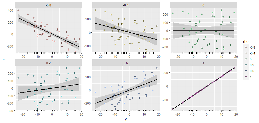
To illustrate, I generated a vector $Y$ with $50$ components and produced various $Z=X_{Y;\rho}$ having specified correlations $\rho$ with this $Y$. They were all created with the same starting vector $X=(1,2,\ldots, 50)$. Here are their $(Y,Z)$ scatterplots. The "rugplots" at the bottom of each panel show the common $Y$ vector.

There's a remarkable similarity among the plots, isn't there :-).

---

If you would like to experiment, modify this code that produced the data and the figure. (I didn't bother to use the freedom to shift and scale the results, which are easy operations.)

y <- rnorm(50, sd=10)
x <- 1:50 # Optional
rho <- seq(0, 1, length.out=6) * rep(c(-1,1), 3)
X <- data.frame(z=as.vector(sapply(rho, function(rho) complement(y, rho, x))),
                rho=ordered(rep(signif(rho, 2), each=length(y))),
                y=rep(y, length(rho)))
    
library(ggplot2)
ggplot(X, aes(y,z, group=rho)) + 
  geom_smooth(method="lm", color="Black") + 
  geom_rug(sides="b") + 
  geom_point(aes(fill=rho), alpha=1/2, shape=21) +
  facet_wrap(~ rho, scales="free")

---

BTW, this method readily generalizes to more than one $Y$: if it's mathematically possible, it will find an $X_{Y_1,Y_2,\ldots,Y_k;\rho_1,\rho_2,\ldots,\rho_k}$ having specified correlations with an entire set of $Y_i$. Just use ordinary least squares to take out the effects of all the $Y_i$ from $X$ and form a suitable linear combination of the $Y_i$ and the residuals. (It helps to do this in terms of a dual basis for $Y$, which is obtained by computing a pseudo-inverse. The following code uses the SVD of $Y$ to accomplish that.)

Here's a sketch of the algorithm in R, where the $Y_i$ are given as columns of a matrix y:

y <- scale(y)             # Makes computations simpler
e <- residuals(lm(x ~ y)) # Take out the columns of matrix `y`
y.dual <- with(svd(y), (n-1)*u %*% diag(ifelse(d > 0, 1/d, 0)) %*% t(v))
sigma2 <- c((1 - rho %*% cov(y.dual) %*% rho) / var(e))
return(y.dual %*% rho + sqrt(sigma2)*e)

Another thread provides a detailed explanation of each line of code. The following is a more complete implementation for those who would like to experiment.

complement <- function(y, rho, x, threshold=1e-12) {
  #
  # Process the arguments.
  #
  if(!is.matrix(y)) y <- matrix(y, ncol=1)
  d <- ncol(y)
  n <- nrow(y)
  y <- scale(y, center=FALSE) # Makes computations simpler
  if (missing(x)) x <- rnorm(n)
  #
  # Remove the effects of `y` on `x`.
  #
  e <- residuals(lm(x ~ y))
  #
  # Calculate the coefficient `sigma` of `e` so that the correlation of
  # `y` with the linear combination y.dual %*% rho + sigma*e is the desired
  # vector.
  #
  y.dual <- with(svd(y), (n-1)*u %*% diag(ifelse(d > threshold, 1/d, 0)) %*% t(v))
  sigma2 <- c((1 - rho %*% cov(y.dual) %*% rho) / var(e))
  #
  # Return this linear combination.
  #
  if (sigma2 >= 0) {
    sigma <- sqrt(sigma2) 
    z <- y.dual %*% rho + sigma*e
  } else {
    warning("Correlations are impossible.")
    z <- rep(0, n)
  }
  return(z)
}
#
# Set up the problem.
#
d <- 3           # Number of given variables
n <- 50          # Dimension of all vectors
x <- 1:n         # Optionally: specify `x` or draw from any distribution
y <- matrix(rnorm(d*n), ncol=d) # Create `d` original variables in any way
rho <- c(0.5, -0.5, 0)          # Specify the correlations
#
# Verify the results.
#
z <- complement(y, rho, x)
cbind('Actual correlations' = cor(y, z),
      'Target correlations' = rho)
#
# Display them.
#
colnames(y) <- paste0("y.", 1:d)
colnames(z) <- "z"
pairs(cbind(z, y))

Answer 3

Here's another computational approach (the solution is adapted from a forum post by Enrico Schumann). According to Wolfgang (see comments), this is computationally identical to the solution proposed by ttnphns.

In contrast to caracal's solution it does not produce a sample with the exact correlation of $\rho$, but two vectors whose population correlation is equal to $\rho$.

Following function can compute a bivariate sample distribution drawn from a population with a given $\rho$. It either computes two random variables, or it takes one existing variable (passed as parameter x) and creates a second variable with the desired correlation:

# returns a data frame of two variables which correlate with a population correlation of rho
# If desired, one of both variables can be fixed to an existing variable by specifying x
getBiCop <- function(n, rho, mar.fun=rnorm, x = NULL, ...) {
     if (!is.null(x)) {X1 <- x} else {X1 <- mar.fun(n, ...)}
     if (!is.null(x) & length(x) != n) warning("Variable x does not have the same length as n!")

     C <- matrix(rho, nrow = 2, ncol = 2)
     diag(C) <- 1

     C <- chol(C)

     X2 <- mar.fun(n)
     X <- cbind(X1,X2)

     # induce correlation (does not change X1)
     df <- X %*% C

     ## if desired: check results
     #all.equal(X1,X[,1])
     #cor(X)

     return(df)
}

The function can also use non-normal marginal distributions by adjusting parameter mar.fun. Note, however, that fixing one variable only seems to work with a normally distributed variable x! (which might relate to Macro's comment).

Also note that the "small correction factor" from the original post was removed as it seems to bias the resulting correlations, at least in the case of Gaussian distributions and Pearson correlations (also see comments).

Answer 4

Let $X$ be your fixed variable and you want to generate $Y$ variable that correlates with $X$ by amount $r$. If $X$ is standardized then (because $r$ is beta coefficient in simple regression) $Y= rX+E$, where $E$ is random variable from normal distribution having mean $0$ and $\text{sd}=\sqrt{1-r^2}$. Observed correlation between $X$ and $Y$ data will be approximately $r$; $X$ and $Y$ can be seen as random samples from bivariate normal population (if $X$ is from normal) with $\rho=r$.

Now, if you want to attain the correlation in your bivariate sample exactly $r$, you need to provide that $E$ has zero correlation with $X$. This tightening it to zero can be reached by modifying $E$ iteratively. Well, with only two variables, one given ($X$) and one to generate ($Y$), the sufficient number of iterations is actually 1, but with multiple given variables ($X_1, X_2, X_3,...$) iterations will be needed.

It should be noted that if $X$ is normal then in the first procedure ("approximate $r$") $Y$ will also be normal; however, in iterative fitting of $Y$ to the "exact $r$" $Y$ is likely to lose normality because the fitting exploits case values selectively.

---

Update Nov 11, 2017. I've come across this old thread today and decided to expand my answer by showing the algorithm of the iterative fitting about which I was speaking initially.

Here is an iterative solution how to train a randomly simulated or preexistent variable $Y$ to correlate or covariate precisely as we desire (or very close to so - depending number of iterations) with a set of given variables $X$s (these cannot be modified).

Disclamer: This iterative solution I've found inferior to the excellent one based on finding the dual basis and proposed by @whuber in this thread today. @whuber's solution is not iterative and, more importantly for me, it seems to be affecting the values of the input "pig" variable somewhat less than "my" algorithm (it'd be an asset then if the task is to "correct" the existing variable and not to generate random variate from scratch). Still, I'm publishing mine for curiosity and because it works (see also Footnote).

So, we have given (fixed) variables $X_1, X_2,...,X_m$, and varible $Y$ which is either just randomly generated "pig" of values or is an existent data variable which values we need to "correct" - to bring $Y$ exactly to correlations (or it can be covariances) $r_1, r_2,...,r_m$ with the $X$s. All data must be continuous; in other words, there should be a good deal of unique values.

The idea: perform iterative fitting of residuals. Knowing the wanted (target) correlations/covariances, we may compute predicted values for the $Y$ using the $X$s as multiple linear predictors. After obtaining the initial residuals (from the current $Y$ and the ideal prediction), train them iteratively not to correlate with the predictors. In the end, regain $Y$ with the residuals. (The procedure was my own experimental invention of the wheel many years ago when I knew none of the theory; I coded it then in SPSS.)

1. Convert the target $r$s to sums-of-crossproducts by multiplying them by $\text{df}=n-1$: $S_j=r_j \text{df}$. ($j$ is a $X$ variable index.)

2. Z-standardize all the variables (center each, then divide by the st. deviation computed on that above $\text{df}$). $Y$ and $X$s are thus standard. Observed sums of squares are now = $\text{df}$.

3. Compute regressional coefficients predicting $Y$ by $X$s according to the target $r$s: $\bf b=(X'X)^{-1} S$.

4. Compute predicted values for $Y$: $\hat{Y}=\bf Xb$.

5. Compute residuals $E=Y-\hat{Y}$.

6. Compute the needed (target) sum of squares for residuals: $SS_S=\text{df}-SS_{\hat {Y}}$.

7. (Begin to iterate.) Compute observed sums of crossproducts between current $E$ and every $X_j$: $C_j= \sum_{i=1}^n E_i X_{ij}$

8. Correct values of $E$ in the aim to bring all $C$s closer to $0$ ($i$ is a case index):

   $$E_i[\text{corrected}]=E_i-\frac{\sum_{j=1}^m C_j X_{ij}} {n\sum_{j=1}^m X_{ij}^2}$$

   (the denominator doesn't change on iterations, compute it in advance)

   Or, alternatively, a more efficient formula additionally insures the mean of $E$ becomes $0$. First, do center $E$ at each iteration prior computation of the $C$s at step 7, then on this step 8 correct as:

   $$E_i[\text{corrected}]=E_i-\frac{\sum_{j=1}^m \frac{C_j X_{ij}^3}{\sum_{i=1}^n X_{ij}^2}} {\sum_{j=1}^m X_{ij}^2}$$

   (again, denominators are known in advance)$^1$

9. Bring $SS_E$ to its target value: $E_i[\text{corrected}]=E_i \sqrt{SS_S/SS_E}$

   Go to step 7. (Do, say, 10-20 iterations; the greater is $m$ the more iterations could be needed. If target $r$s were realistic, $SS_S$ is positive, and if sample size $n$ isn't too few, iterations always direct to convergence. End iterating.)

10. Ready: All the $C$s are almost zero now which means the residuals $E$ has been trained to restore target $r$s. Compute the fitting $Y$: $Y[\text{corrected}]=\hat{Y}+E$.

11. The obtained $Y$ is almost standardized. As a last stroke, you may want to standardize it precisely, again like you did it on step 2.

12. You may supply $Y$ with any variance and mean you like. Actually, among the four statistics - min, max, mean, st. dev. - you may select any two values and linearly transform the variable so it posesses them without altering the $r$s (correlations) you've attained (it is all called linear rescaling).

To warn again what was said above. With that pulling of $Y$ exactly to the $r$, the output $Y$ does not have to be normally distributed.

---

$^1$ The correction formula can be further sophisticated, for example, to insure greater homoscedasticity (in terms of sums-of-squares) of $Y$ with every $X$ as well, simultaneously with attaining the correlations, - I've implemented a code for that too. (I don't know if such "double" task is solvable via a more neat - noniterative - approach such as whuber's.)

Answer 5

I felt like doing some programming, so I took @Adam's deleted answer and decided to write a nice implementation in R. I focus on using a functionally oriented style (i.e. lapply style looping). The general idea is to take two vectors, randomly permute one of the vectors until a certain correlation has been reached between them. This approach is very brute-force, but is simple to implement.

First we create a function that randomly permutes the input vector:

randomly_permute = function(vec) vec[sample.int(length(vec))]
randomly_permute(1:100)
  [1]  71  34   8  98   3  86  28  37   5  47  88  35  43 100  68  58  67  82
 [19]  13   9  61  10  94  29  81  63  14  48  76   6  78  91  74  69  18  12
 [37]   1  97  49  66  44  40  65  59  31  54  90  36  41  93  24  11  77  85
 [55]  32  79  84  15  89  45  53  22  17  16  92  55  83  42  96  72  21  95
 [73]  33  20  87  60  38   7   4  52  27   2  80  99  26  70  50  75  57  19
 [91]  73  62  23  25  64  51  30  46  56  39

...and create some example data

vec1 = runif(100)
vec2 = runif(100)

...write a function that permutes the input vector, and correlates it to a reference vector:

permute_and_correlate = function(vec, reference_vec) {
    perm_vec = randomly_permute(vec)
    cor_value = cor(perm_vec, reference_vec)
    return(list(vec = perm_vec, cor = cor_value))
  }
permute_and_correlate(vec2, vec1)
$vec
  [1] 0.79072381 0.23440845 0.35554970 0.95114398 0.77785348 0.74418811
  [7] 0.47871491 0.55981826 0.08801319 0.35698405 0.52140366 0.73996913
 [13] 0.67369873 0.85240338 0.57461506 0.14830718 0.40796732 0.67532970
 [19] 0.71901990 0.52031017 0.41357545 0.91780357 0.82437619 0.89799621
 [25] 0.07077250 0.12056045 0.46456652 0.21050067 0.30868672 0.55623242
 [31] 0.84776853 0.57217746 0.08626022 0.71740151 0.87959539 0.82931652
 [37] 0.93903143 0.74439384 0.25931398 0.99006038 0.08939812 0.69356590
 [43] 0.29254936 0.02674156 0.77182339 0.30047034 0.91790830 0.45862163
 [49] 0.27077191 0.74445997 0.34622648 0.58727094 0.92285322 0.83244284
 [55] 0.61397396 0.40616274 0.32203732 0.84003379 0.81109473 0.50573325
 [61] 0.86719899 0.45393971 0.19701975 0.63877904 0.11796154 0.26986325
 [67] 0.01581969 0.52571331 0.27087693 0.33821824 0.52590383 0.11261002
 [73] 0.89840404 0.82685046 0.83349287 0.46724807 0.15345334 0.60854785
 [79] 0.78854984 0.95770015 0.89193212 0.18885955 0.34303707 0.87332019
 [85] 0.08890968 0.22376395 0.02641979 0.43377516 0.58667068 0.22736077
 [91] 0.75948043 0.49734797 0.25235660 0.40125309 0.72147500 0.92423638
 [97] 0.27980561 0.71627101 0.07729027 0.05244047

$cor
[1] 0.1037542

...and iterate a thousand times:

n_iterations = lapply(1:1000, function(x) permute_and_correlate(vec2, vec1))

Note that R's scoping rules ensure that vec1 and vec2 are found in the global environment, outside the anonymous function used above. So, the permutations are all relative to the original test datasets we generated.

Next, we find the maximum correlation:

cor_values = sapply(n_iterations, '[[', 'cor')
n_iterations[[which.max(cor_values)]]
$vec
  [1] 0.89799621 0.67532970 0.46456652 0.75948043 0.30868672 0.83244284
  [7] 0.86719899 0.55623242 0.63877904 0.73996913 0.71901990 0.85240338
 [13] 0.81109473 0.52571331 0.82931652 0.60854785 0.19701975 0.26986325
 [19] 0.58667068 0.52140366 0.40796732 0.22736077 0.74445997 0.40125309
 [25] 0.89193212 0.52031017 0.92285322 0.91790830 0.91780357 0.49734797
 [31] 0.07729027 0.11796154 0.69356590 0.95770015 0.74418811 0.43377516
 [37] 0.55981826 0.93903143 0.30047034 0.84776853 0.32203732 0.25235660
 [43] 0.79072381 0.58727094 0.99006038 0.01581969 0.41357545 0.52590383
 [49] 0.27980561 0.50573325 0.92423638 0.11261002 0.89840404 0.15345334
 [55] 0.61397396 0.27077191 0.12056045 0.45862163 0.18885955 0.77785348
 [61] 0.23440845 0.05244047 0.25931398 0.57217746 0.35554970 0.34622648
 [67] 0.21050067 0.08890968 0.84003379 0.95114398 0.83349287 0.82437619
 [73] 0.46724807 0.02641979 0.71740151 0.74439384 0.14830718 0.82685046
 [79] 0.33821824 0.71627101 0.77182339 0.72147500 0.08801319 0.08626022
 [85] 0.87332019 0.34303707 0.45393971 0.47871491 0.29254936 0.08939812
 [91] 0.35698405 0.67369873 0.27087693 0.78854984 0.87959539 0.22376395
 [97] 0.02674156 0.07077250 0.57461506 0.40616274

$cor
[1] 0.3166681

...or find the closest value to a correlation of 0.2:

n_iterations[[which.min(abs(cor_values - 0.2))]]
$vec
  [1] 0.02641979 0.49734797 0.32203732 0.95770015 0.82931652 0.52571331
  [7] 0.25931398 0.30047034 0.55981826 0.08801319 0.29254936 0.23440845
 [13] 0.12056045 0.89799621 0.57461506 0.99006038 0.27077191 0.08626022
 [19] 0.14830718 0.45393971 0.22376395 0.89840404 0.08890968 0.15345334
 [25] 0.87332019 0.92285322 0.50573325 0.40796732 0.91780357 0.57217746
 [31] 0.52590383 0.84003379 0.52031017 0.67532970 0.83244284 0.95114398
 [37] 0.81109473 0.35554970 0.92423638 0.83349287 0.34622648 0.18885955
 [43] 0.61397396 0.89193212 0.74445997 0.46724807 0.72147500 0.33821824
 [49] 0.71740151 0.75948043 0.52140366 0.69356590 0.41357545 0.21050067
 [55] 0.87959539 0.11796154 0.73996913 0.30868672 0.47871491 0.63877904
 [61] 0.22736077 0.40125309 0.02674156 0.26986325 0.43377516 0.07077250
 [67] 0.79072381 0.08939812 0.86719899 0.55623242 0.60854785 0.71627101
 [73] 0.40616274 0.35698405 0.67369873 0.82437619 0.27980561 0.77182339
 [79] 0.19701975 0.82685046 0.74418811 0.58667068 0.93903143 0.74439384
 [85] 0.46456652 0.85240338 0.34303707 0.45862163 0.91790830 0.84776853
 [91] 0.78854984 0.05244047 0.58727094 0.77785348 0.01581969 0.27087693
 [97] 0.07729027 0.71901990 0.25235660 0.11261002

$cor
[1] 0.2000199

To get a higher correlation, you need to increase the number of iterations.

Answer 6

Let's solve a more general problem: given variable $Y_1$ how to generate the random variables $Y_2,\dots,Y_n$ with correlation matrix $R$?

Solution:

1. get the cholesky decomposition of the correlation matrix $CC^T=R$
2. create independent random vectors $X_2,\dots,X_n$ of the same length as $Y_1$
3. Use $Y_1$ as the first column and append the generated randoms to it
4. $Y=CX$, where $Y_i$ - the new random correlated numbers as required, note, that $Y_1$ will not change

Python code:

import numpy as np
import math
from scipy.linalg import toeplitz, cholesky
from statsmodels.stats.moment_helpers import cov2corr

# create the large correlation matrix R
p = 4
h = 2/p
v = np.linspace(1,-1+h,p)
R = cov2corr(toeplitz(v))

# create the first variable
T = 1000;
y = np.random.randn(T)

# generate p-1 correlated randoms
X = np.random.randn(T,p)
X[:,0] = y
C = cholesky(R)
Y = np.matmul(X,C)

# check that Y didn't change
print(np.max(np.abs(Y[:,0]-y)))

# check the correlation matrix
print(R)
print(np.corrcoef(np.transpose(Y)))

Test Output:

0.0
[[ 1.   0.5  0.  -0.5]
 [ 0.5  1.   0.5  0. ]
 [ 0.   0.5  1.   0.5]
 [-0.5  0.   0.5  1. ]]
[[ 1.          0.50261766  0.02553882 -0.46259665]
 [ 0.50261766  1.          0.51162821  0.05748082]
 [ 0.02553882  0.51162821  1.          0.51403266]
 [-0.46259665  0.05748082  0.51403266  1.        ]]

Answer 7

Equivalent Python answer to @caracal 's :

import math
import numpy as np
import scipy.stats as ss
from scipy import linalg

n = 20 # length of vector
rho = 0.6 # desired correlation = cos(angle)
theta = math.acos(rho)# corresponding angle

mu1=3
sigma1 = 0.5

mu2= 2
sigma2=0.2


x1 = np.random.normal(mu1, sigma1, n)
x2 = np.random.normal(mu2, sigma2, n)
X = np.vstack((x1,x2)).T

Xctr = ss.zscore(X) # centered columns (mean 0)
Id = np.diag(np.ones(n)) # identity matrix
Q = np.linalg.qr(Xctr)[0][:,0]# QR-decomposition, just matrix Q
P = Q.reshape(-1, 1) @ Q.reshape(1, -1) # projection onto space defined by x1
x2o = (Id-P) @ Xctr[ :, 1]  # x2ctr made orthogonal to x1ctr
Xc2 = np.vstack((Xctr[:,0], x2o)).T # bind to matrix
Y = Xc2 @ np.diag(1/np.sum(Xc2**2, axis=0)**0.5) # scale columns to length 1
x = Y[ :, 1] + (1 / math.tan(theta)) * Y[:,0] # final new vector
np.corrcoef((x1, x))[0,1]  # check correlation = rho

Answer 8

Generate normal variables with SAMPLING covariance matrix as given

covsam <- function(nobs,covm, seed=1237) {; 
          library (expm);
          # nons=number of observations, covm = given covariance matrix ; 
          nvar <- ncol(covm); 
          tot <- nvar*nobs;
          dat <- matrix(rnorm(tot), ncol=nvar); 
          covmat <- cov(dat); 
          a2 <- sqrtm(solve(covmat)); 
          m2 <- sqrtm(covm);
          dat2 <- dat %*% a2 %*% m2 ; 
          rc <- cov(dat2);};
          cm <- matrix(c(1,0.5,0.1,0.5,1,0.5,0.1,0.5,1),ncol=3);
          cm; 
          res <- covsam(10,cm)  ;
          res;

Generate normal variables with POPULATION covariance matrix as given

covpop <- function(nobs,covm, seed=1237) {; 
          library (expm); 
          # nons=number of observations, covm = given covariance matrix;
          nvar <- ncol(covm); 
          tot <- nvar*nobs;  
          dat <- matrix(rnorm(tot), ncol=nvar); 
          m2 <- sqrtm(covm);
          dat2 <- dat %*% m2;  
          rc <- cov(dat2); }; 
          cm <- matrix(c(1,0.5,0.1,0.5,1,0.5,0.1,0.5,1),ncol=3);
          cm; 
          res <- covpop(10,cm); 
          res

Answer 9

Given:

$\rho$ = desired correlation between Y and Z
$Z$ = sample

Requested:

'Random' sample $Y$ such that $cor(Y, Z) = \rho$

Solution:

Let $x_1 =$ scale($Z$), which implies $E(x_1) = 0, Var(x_1) = 1$
Generate a random sample $x_2$ with $E(x_2) = 0$ and $Var(x_2) = 1$ (distribution not important)
We then determine scalar $a$ such that $Y = x_1 + a * x_2$ satisfies the requirement.
Let $cv = cov(x_1, x_2)$.
We then have:
\begin{eqnarray*} Var(Y) &=& Var(x_1 + a * x_2) \\ &=& Var(x_1) + a^2 * Var(x_2) + 2 * a * cov(x_1, x_2) \\ &=& 1 + a^2 + 2*a*cv \\ cor(Y, Z) &=& cor(Y, x_1) \\ &=& cov(x_1 + a * x_2, x_1) / sqrt(Var(Y)*Var(x_1)) \\ &=& [Var(x_1) + a * cov(x_2, x_1)] / sqrt(1 + a^2 + 2*a*cv)\\ &=& (1 + a * cv) / sqrt(1 + a^2 + 2*a*cv) \end{eqnarray*} So
\begin{eqnarray*} \rho * sqrt(1 + a^2 + 2*a*cv) &=& (1 + a * cv) \\ \rho^2 * (1 + a^2 + 2 * a * cv) &=& (1 + a * cv)^2 \\ \rho^2 + \rho^2 * a^2 + 2 * cv * \rho^2 * a &=& 1 + 2 * cv * a + cv^2 * a^2\\ a^2 * (\rho^2 - cv^2) + 2 * a * (cv * \rho^2 - cv) + \rho^2 - 1 &=& 0\\ a^2 * (\rho^2 - cv^2) - 2 * a * cv * (1 - \rho^2) - (1 - \rho^2) &=& 0\\ \end{eqnarray*} We remember from the second line above that $sign(\rho) = sign(1 + a * cv)$.
Solving the quadratic equation:
\begin{eqnarray*} \Delta &=& cv^2 * (1 - \rho^2)^2 + (1 - \rho^2) * (\rho^2 - cv^2) \\ &=& (1 - \rho^2) * [cv^2 * (1 - \rho^2) + \rho^2 - cv^2] \\ &=& (1 - \rho^2) * \rho^2 * (1 - cv^2) \\ a &=& [cv * (1 - \rho^2) \pm \sqrt \Delta ] / [\rho^2-cv^2] \\ \end{eqnarray*} This gives an r-function, about 2.5 times faster then the beautiful 'complement' function (solution by whuber):\

corr <- function(z, rho){ \
  x1 <- c(scale(z)) \
  x2 <- scale(rnorm(length(x1))) \
  cv <-c(cov(x2, x1)) \
  sqrtdelta <- sqrt(rho^2 * (1 - rho^2) * (1 - cv^2)) \
  a <- (sqrtdelta + cv * (1-rho^2)) / (rho^2 - cv^2) \
  if (correlation * (1 + a * cv) < 0) a <- (-sqrtdelta + cv * (1-rho^2)) / (rho^2 - cv^2) \
  a * x2 + x1 \
}