Interpretation of Hartigans' dip test

Question

I would like to find a way to quantify the intensity of bimodality of some distributions I got empirically. From what I read, there is still some debate about the way to quantify bimodality. I chose to use Hartigans' dip test which seems to be the only one available on R (original paper : http://www.stat.washington.edu/wxs/Stat593-s03/Literature/hartigan85a.pdf). Hartigans' dip test is defined as : "The dip test measures multimodality in a sample by the maximum difference, over all sample points, between the empirical distribution function, and the unimodal distribution function that minimizes that maximum difference".

I would like to understand completely how I should interpret this statistics before using it. I was expecting that the dip test would increase if the distribution is multimodal (as it is defined as "the maximum difference from the unimodal distribution"). But : you can read in the wikipedia page about multimodal distribution that "Values less than 0.05 indicate significant bimodality and values greater than 0.05 but less than 0.10 suggest bimodality with marginal significance.". Such statement comes from this paper (Fig. 2). According this paper, the dip test index is close to 0 when the distribution is bimodal. It confuses me.

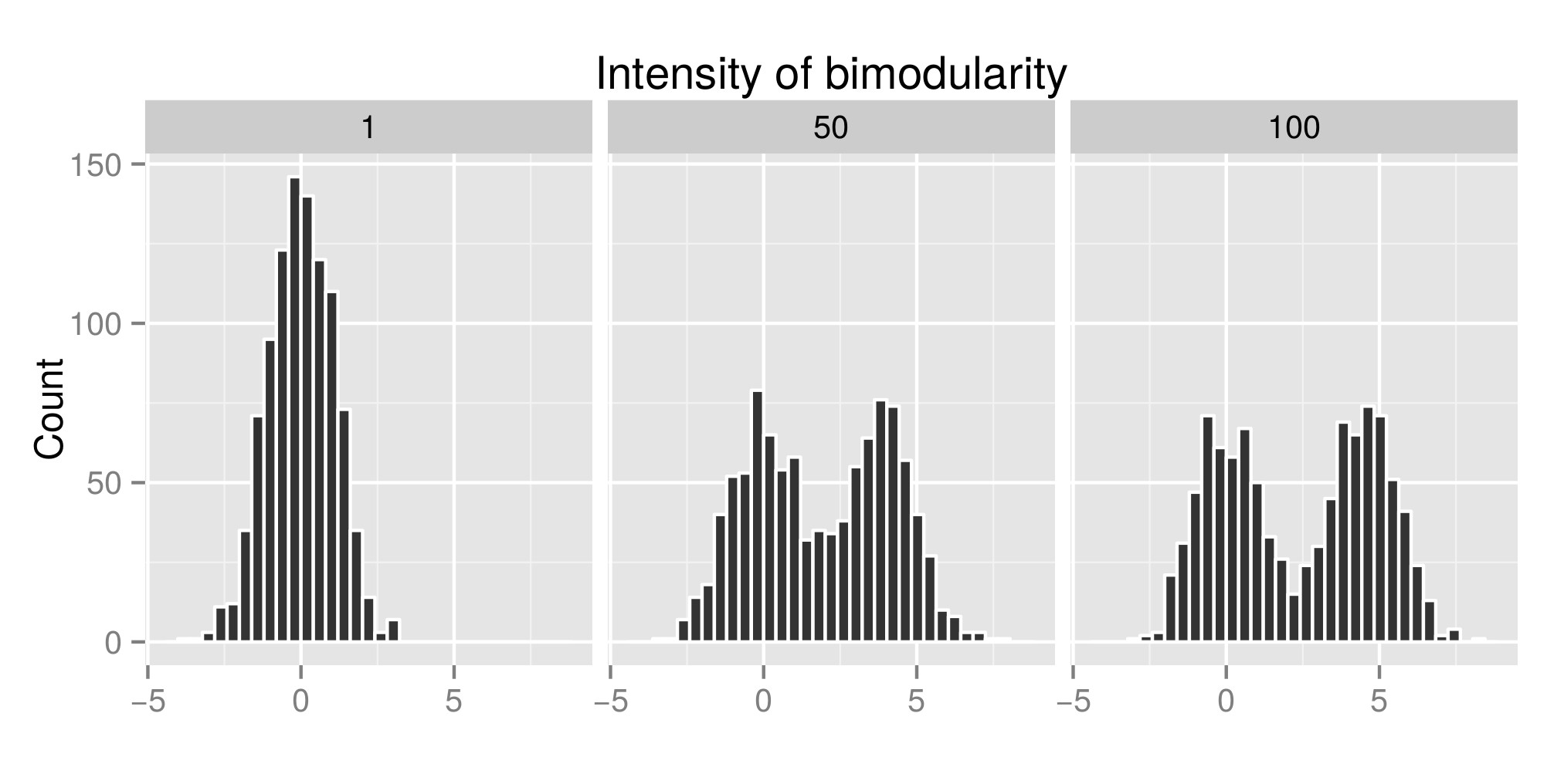
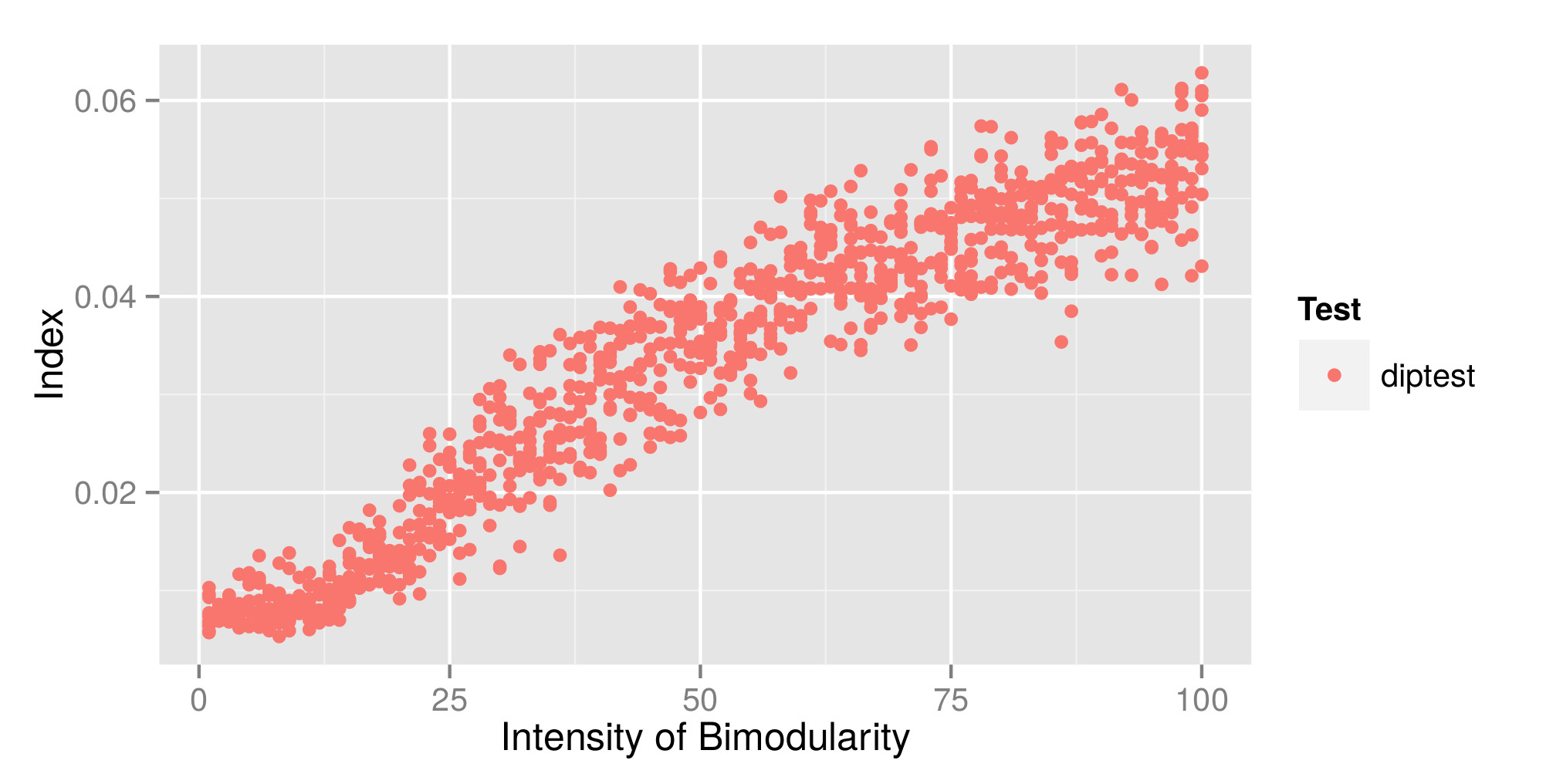
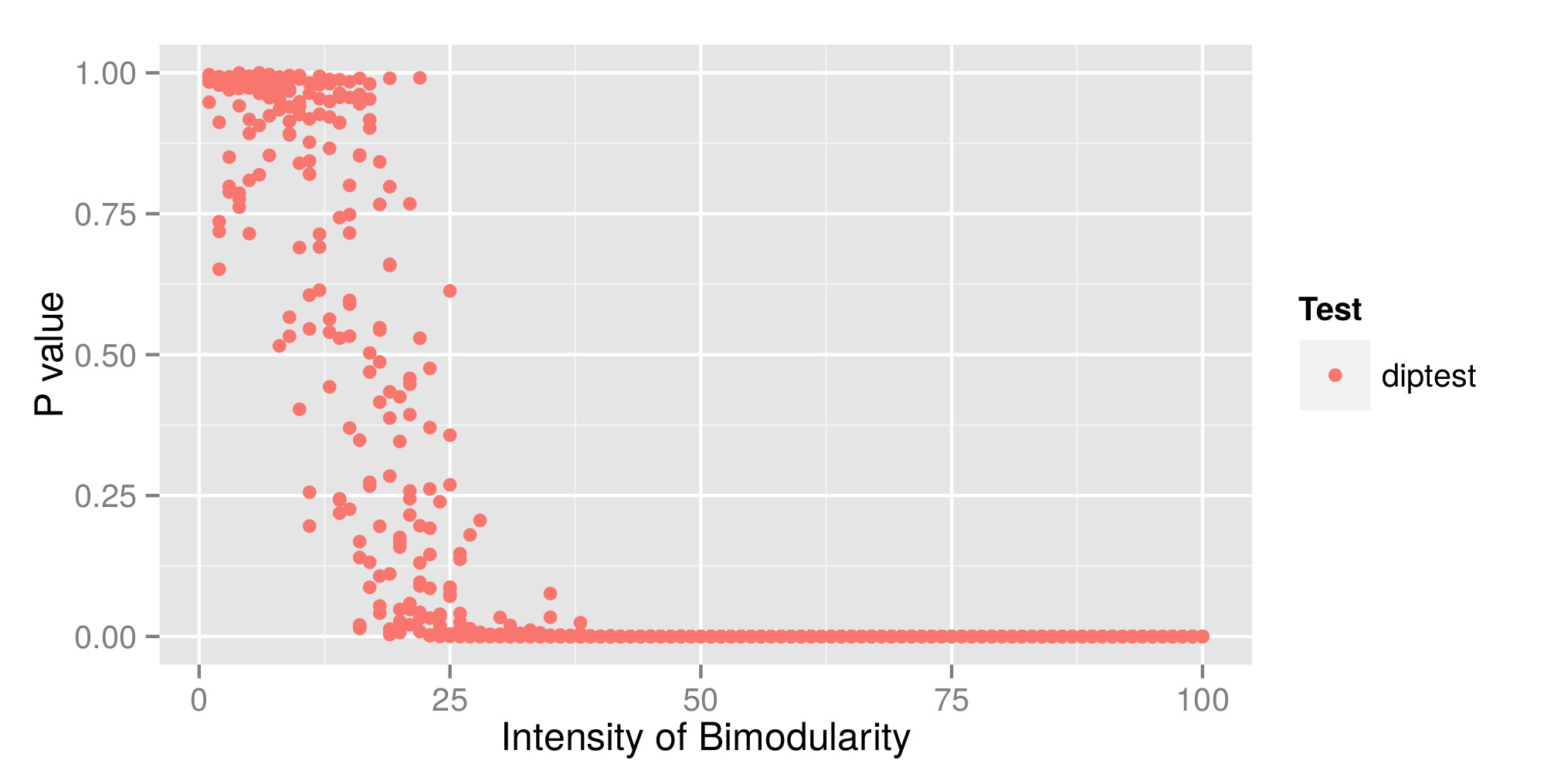
To interpret correctly the Hartigans' dip test I constructed some distributions (the original code is from here) and I increased the value of exp(mu2) (called 'Intensity of bimodularity' from now on - Edit : I should have called it 'Intensity of bimodality') to get bimodality. In the first graph, you can see some example of distributions. Then I estimated the diptest index (second graph) and the p value (third graphe) associated (package diptest) to those different simulated distributions. The R code used is at the end of my post.

What I show here is that the dip test index is high and the Pvalue is low when the distibutions are bimodal. Which is contrary to what you can read on the internet.

I am no expert in statistics, so that I barely understood Hartigans' paper. I would like to get some comments about the right way we should interpret Hartigans' dip test. Am I wrong somewhere ?

Thank you all. Regards,

T.A.

Example of distribution simulated :

Hartigan's dip test index associated :

Hartigan's dip test p.value associated :

library(diptest)
library(ggplot2)


# CONSTANT PARAMETERS
sig1 <- log(3)
sig2 <- log(3)
cpct <- 0.5
N=1000

#CREATING BIMOD DISTRIBUTION
bimodalDistFunc <- function (n,cpct, mu1, mu2, sig1, sig2) {
  y0 <- rlnorm(n,mean=mu1, sd = sig1)
  y1 <- rlnorm(n,mean=mu2, sd = sig2)

  flag <- rbinom(n,size=1,prob=cpct)
  y <- y0*(1 - flag) + y1*flag 
}

#DIP TEST
DIP_TEST <- function(bimodalData) {
  TEST <- dip.test(bimodalData)
  return(TEST$statistic[[1]])   # return(TEST$p.value[[1]])    to get the p value
}
DIP_TEST(bimodalData)


# SIMULATION
exp_mu1 = 1
max_exp_mu2 = 100
intervStep = 100
repPerInt = 10

# single distibutions
expMu2Value <- c()
bimodalData <- c()
mu1 <- log(exp_mu1)   
mu2 <- log(exp_mu1)
bimodalData <- c(bimodalData,log(bimodalDistFunc(n=N,cpct,mu1,mu2, sig1,sig2)))
expMu2Value <- c(expMu2Value,rep(exp_mu1,length(log(bimodalDistFunc(n=N,cpct,mu1,mu2, sig1,sig2)))))

mu1 <- log(exp_mu1)   
mu2 <- log(max_exp_mu2)
bimodalData <- c(bimodalData,log(bimodalDistFunc(n=N,cpct,mu1,mu2, sig1,sig2)))
expMu2Value <- c(expMu2Value,rep(max_exp_mu2,length(log(bimodalDistFunc(n=N,cpct,mu1,mu2, sig1,sig2)))))

mu1 <- log(exp_mu1)   
mu2 <- log(trunc((max_exp_mu2-exp_mu1)/2+1))
bimodalData <- c(bimodalData,log(bimodalDistFunc(n=N,cpct,mu1,mu2, sig1,sig2)))
expMu2Value <- c(expMu2Value,rep(trunc((max_exp_mu2-exp_mu1)/2+1),length(log(bimodalDistFunc(n=N,cpct,mu1,mu2, sig1,sig2)))))

tableExamples <- data.frame(expMu2Value,bimodalData)
tableExamples$expMu2Value <- as.factor(tableExamples$expMu2Value)
ExamplePlot <- ggplot(tableExamples)+
  geom_histogram(aes(bimodalData),color='white')+
  ylab("Count")+
  xlab("")+
  facet_wrap(~expMu2Value)+
  ggtitle("Intensity of bimodularity")

# calculation of the dip test index
exp_mu2Int = seq(from=exp_mu1,to=max_exp_mu2,length.out=intervStep)
expmu2Vec = c()
dipStat = c()
testDone = c()
for(exp_mu2 in exp_mu2Int){
  mu1 <- log(exp_mu1)   
  mu2 <- log(exp_mu2)
  for(rep in 1:repPerInt){
    bimodalData <- log(bimodalDistFunc(n=N,cpct,mu1,mu2, sig1,sig2))
    diptestone = DIP_TEST(bimodalData)
    expmu2Vec = c(expmu2Vec,exp_mu2)
    dipStat = c(dipStat,diptestone)
    testDone = c(testDone,"diptest")
  }
}
table = data.frame(expmu2Vec,dipStat,testDone)

IndexPlot <- ggplot(table)+
  geom_point(aes(expmu2Vec,dipStat,color=testDone))+
  ylab("Index")+
  xlab("Intensity of Bimodularity")+
  scale_color_discrete(name="Test")

ExamplePlot
IndexPlot

Answer 1

Mr. Freeman (author of the paper I told you about) told me that he was actually looking only at the Pvalue of the dip test. This confusion comes from his sentence :
"HDS values range from 0 to 1 with values less than .05 indicating significant bimodality, and values greater than .05 but less than .10 suggesting bimodality with marginal significance". HDS values corresponds to the Pvalue, and not the dip test statistics. It was unclear in the paper.

My analysis is good : the dip test statistics increases when the distribution is deviant from a unimodal distribution.

Bimodality test and Silverman's test can also be computed easily in R and do the job well.