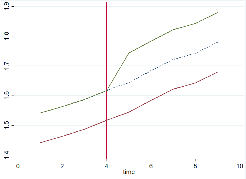
The typical thing to do is visual inspection of the pre-treatment trends for the control and treatment group. This is particularly easy if you only have those two groups given a single binary treatment. Ideally the pre-treatment trends should look something like this:

This graph was taken from a previous answer to the question why we need the common trends assumption. This includes also an explanation of the blue-dashed line which is the counterfactual outcome for the treated that can be assumed if we can reasonably verify the parallel trends assumption.
A formal test which is also suitable for multivalued treatments or several groups is to interact the treatment variable with time dummies. Suppose you have 3 pre-treatment periods and 3 post-treatment periods, you would then regress
$$y_{it} = \lambda_i + \delta_t + \beta_{-2}D_{it} + \beta_{-1}D_{it} + \beta_1 D_{it} + \beta_2 D_{it} + \beta_3 D_{it} + \epsilon_{it}$$
where $y$ is the outcome for individual $i$ at time $t$, $\lambda$ and $\delta$ are individual and time fixed effects (this is a generalized way of writing down the diff-in-diff model which also allows for multiple treatments or treatments at different times).
The idea is the following. You include the interactions of the time dummies and the treatment indicator for the first two pre-treatment periods and you leave out the one interaction for the last pre-treatment period due to the dummy variable trap. Also now all the other interactions are expressed relative to the omitted period which serves as the baseline. If the outcome trends between treatment and control group are the same, then $\beta_{-2}$ and $\beta_{-1}$ should be insignificant, i.e. the difference in differences is not significantly different between the two groups in the pre-treatment period.
An attractive feature of this test is that also the interactions of the time dummies after the treatment with the treatment indicator is informative. For instance, $\beta_{1}, \beta_2, \beta_3$ show you whether the treatment effect fades out over time, stays constant, or even increases. An application of this approach is Autor (2003).
Note that the literature generally refers to $\beta_{-2}, \beta_{-1}$ as "leads" and $\beta_{1}, \beta_2, \beta_3$ as "lags", even though they are merely interactions of the treatment indicator with time dummies and are not actually leads and lags of the treatment indicator in a time-series jargon sense. A more detailed explanation of this parallel trends test is provided in the lecture notes by Steve Pischke (here on page 7, or here on page 9).

