3
$\begingroup$
library(muhaz)
nsam = 5000
time <- rexp(nsam,4)
cause0 = rbinom(nsam,1,.75)
haz = muhaz(time,cause0)
plot(haz)
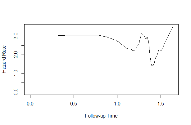
enter image description here

I simulated failure time data which is exponentially distributed with parameter 4 and the proportion of non-censoring is 75%. Using 'muhaz' function, I expected that the estimate of hazard is close to 4 which is the exponential parameter regardless of censoring. But it is around 3 which seems to be 4 * 0.75. Since the censoring indicators were independently generated from the failure time data, I believe that the estimates of hazard should be constantly 4 regardless of the proportion of censoring.

Am I misunderstanding something or did something go wrong in muhaz function?

$\endgroup$
3
  • 1
    $\begingroup$ If you censor 25% of the cases, then they contribute exposure time up until the censoring-"event", but they do not contribute to the numerator of the rate. So you have decreased the real events by 25% but not the exposure time. As you decrease the censoring proportion, the rate estimate approaches 4. $\endgroup$
    – DWin
    Commented Jul 18, 2015 at 6:49
  • $\begingroup$ Probably a better fit for stats.stackexchange... $\endgroup$ Commented Jul 18, 2015 at 7:29
  • 1
    $\begingroup$ The reason I didn't vote to migrate is that I thought it was an effort at a bug report (or a bug question anyway.) Since I'm the maintainer of pkg:muhaz, I thought that my reply was sufficient, but if the questioner had further need of clarification I was prepared to actually do some coding. (It's not true that the censoring indicators were independent of the times. They were in fact completely dependent on the times. It's as if 25% of the cases were censored just before they died.) $\endgroup$
    – DWin
    Commented Jul 18, 2015 at 17:13

1 Answer 1

3
$\begingroup$

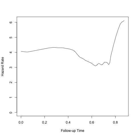
When you censor by simply choosing to randomly change the censoring variable, you are essentially leaving in all of the case-"times" under observation until just before they would have died during a complete observation model. (That is an egregious violation of the non-informative censoring assumption needed for survival analysis.) You need to change this to a model where the censoring process shortens time to a sensible (random) number for the censored cases.

censRand <- function(time, cens.t.5){  # cens.t.5 is the t 1/2 of censor process
  ctime <- rexp(n = length(time), rate = 1/cens.t.5)
  event <- (time <= ctime)
  t_obs <- pmin(time, ctime)
  return(data.frame(Times=t_obs, event=event))
}

time=rexp(1000, 4)
ctime <- censRand( time, 0.7)
plot( muhaz( ctime[ ,1], ctime[,2]) )

enter image description here

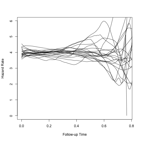
To get a further notion of the range of time over which this might be a "stable" estimate (if it were not already apparent from the excursions around the simulated parameter) you can run it multiple times:

png()
 plot( muhaz( ctime[ ,1], ctime[,2]) );
 for (i in 1:20) { time=rexp(1000, 4)
                    ctime <- censRand( time, 0.7)
                    lines( muhaz( ctime[ ,1], ctime[,2]) ) };
dev.off()

enter image description here

$\endgroup$

Your Answer

By clicking “Post Your Answer”, you agree to our terms of service and acknowledge you have read our privacy policy.

Not the answer you're looking for? Browse other questions tagged or ask your own question.