What's the difference between logistic regression and perceptron?

Question

I'm going through Andrew Ng's lecture notes on Machine Learning.

The notes introduce us to logistic regression and then to perceptron. While describing Perceptron, the notes say that we just change the definition of the threshold function used for logistic regression. After doing that, we can use the Perceptron model for classification.

So my question is - if this needs to be specified and we consider Perceptron as a classification technique, then what exactly is logistic regression? Is is just used to get the probability of a data point belonging to one of the classes?

Answer 1

In short, logistic regression has probabilistic connotations that go beyond the classifier use in ML. I have some notes on logistic regression here.

The hypothesis in logistic regression provides a measure of uncertainty in the occurrence of a binary outcome based on a linear model. The output is bounded asymptotically between $0$ and $1$, and depends on a linear model, such that when the underlying regression line has value $0$, the logistic equation is $0.5 = \frac{e^0}{1+e^0}$, providing a natural cutoff point for classification purposes. However, it is at the cost of throwing out the probability information in the actual result of $h(\Theta^T\bf x) =\frac{e^{\Theta^T \bf x}}{1 +e^{\Theta^T\bf x}}$, which often is interesting (e.g. probability of loan default given income, credit score, age, etc.).

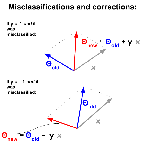
The perceptron classification algorithm is a more basic procedure, based on dot products between examples and weights. Whenever an example is misclassified the sign of the dot product is at odds with the classification value ($-1$ and $1$) in the training set. To correct this, the example vector will be iteratively added or subtracted from the vector of weights or coefficients, progressively updating its elements:

Vectorially, the $d$ features or attributes of an example are $\bf x$, and the idea is to "pass" the example if:

$\displaystyle \sum_{1}^d \theta_i x_i > \text{theshold}$ or...

$h(x) = \text{sign}\big(\displaystyle \sum_{1}^d \theta_i x_i - \text{theshold}\big)$. The sign function results in $1$ or $-1$, as opposed to $0$ and $1$ in logistic regression.

The threshold will be absorbed into the bias coefficient, $+ \theta_0$. The formula is now:

$h(x) = \text{sign}\big(\displaystyle \sum_0^d \theta_i x_i\big)$, or vectorized: $h(x) = \text{sign}(\theta^T\bf x)$.

Misclassified points will have $\text{sign}(\theta^T\bf x) \neq y_n$, meaning that the dot product of $\Theta$ and $\bf x_n$ will be positive (vectors in the same direction), when $y_n$ is negative, or the dot product will be negative (vectors in opposite directions), while $y_n$ is positive.

---

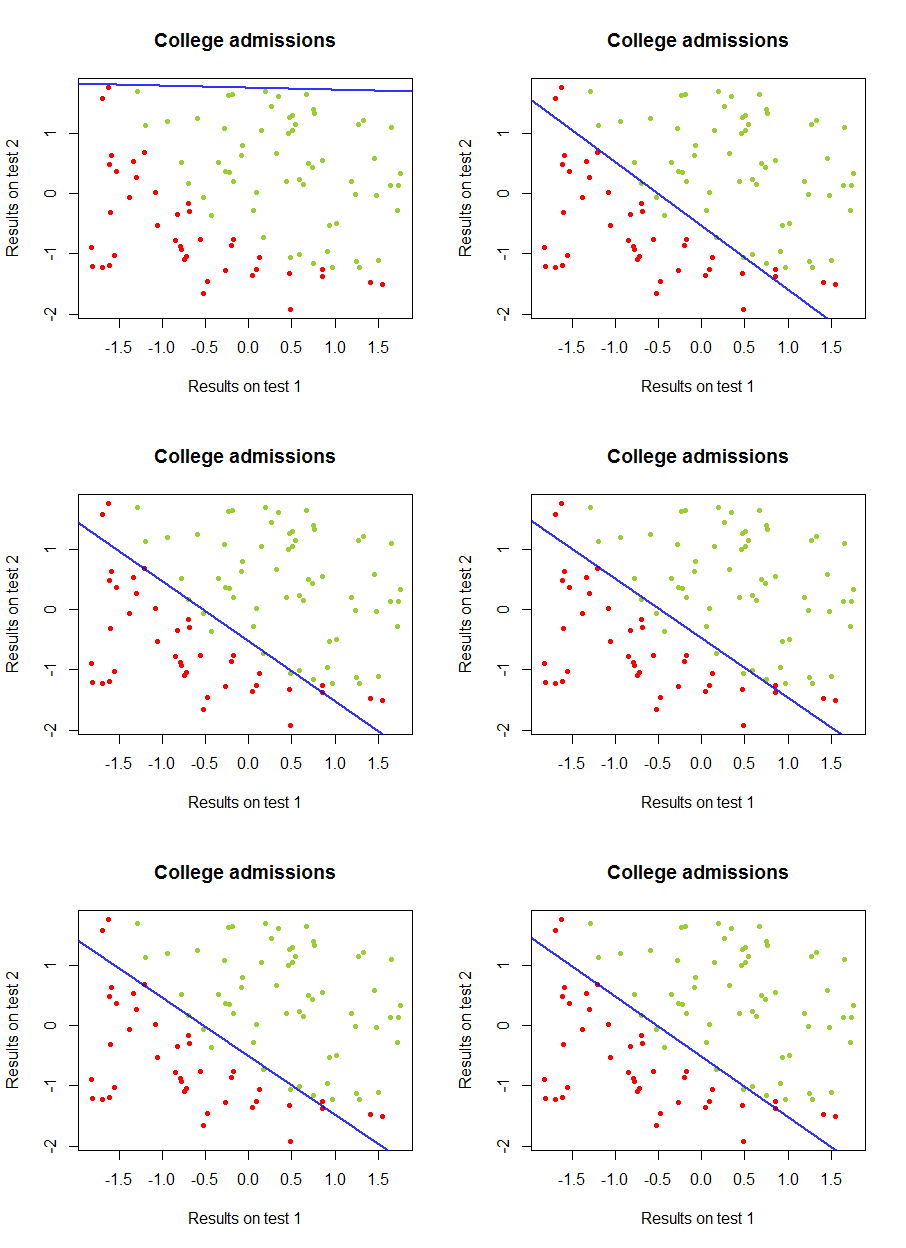
I have been working on the differences between these two methods in a dataset from the same course, in which the test results in two separate exams are related to the final acceptance to college:

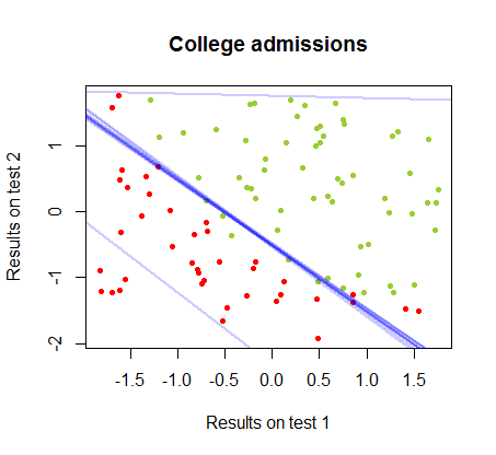
The decision boundary can be easily found with logistic regression, but was interesting to see that although the coefficients obtained with perceptron were vastly different than in logistic regression, the simple application of the $\text{sign}(\cdot)$ function to the results yielded just as good a classifying algorithm. In fact the maximum accuracy (the limit set by linear inseparability of some examples) was reached by the second iteration. Here is the sequence of boundary division lines as $10$ iterations approximated the weights, starting from a random vector of coefficients:

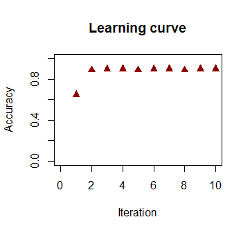
The accuracy in the classification as a function of the number of iterations increases rapidly and plateaus at $90\%$, consistent how fast a near-optimal decision boundary is reached in the videoclip above. Here is the plot of the learning curve:

---

The code used is here.

Answer 2

There is some confusion that may arise here. Originally a perceptron was only referring to neural networks with a step function as the transfer function. In that case of course the difference is that the logistic regression uses a logistic function and the perceptron uses a step function. In general both algorithm should yield the same decision boundary (at least for a single neuron perceptron). However:

1. The parameter vector for the perceptron may be arbitrarily scaled compared to the one derived by logistic regression. Any scaling of the parameter vector will define the same boundary, but the probabilities calculated by logistic regression depend on the exact scaling.
2. The output from a step function can of course not be interpreted as any kind of probability.
3. Since a step function is not differentiable, it is not possible to train a perceptron using the same algorithms that are used for logistic regression.

In some cases, the term perceptron is also used to refer to neural networks which use a logistic function as a transfer function (however, this is not in accordance with the original terminology). In that case, a logistic regression and a "perceptron" are exactly the same. Of course, with a perceptron it is possible to use multiple neurons all using a logistic transfer function, which becomes somewhat relatable to stacking of logistic regression (not the same, but similar).

Answer 3

You can use logistic regression to build a perceptron. The logistic regression uses logistic function to build the output from a given inputs. Logistic function produces a smooth output between 0 and 1, so you need one more thing to make it a classifier, which is a threshold. Perceptrons can be built with other functional forms, of course, not just logistic.

The logistic regression produces you the model that looks like this: $$y(x_1,x_2|b)=\frac{e^{b_0+b_1x_1+b_2x_2}}{1+e^{b_0+b_1x_1+b_2x_2}}$$ The regression part is how to estimate the coefficients $b_1,b_2,b_3$, the logistic part is the function form $\frac{e^x}{1+e^x}$

Once you calculate $y(x|b)$ given inputs $x$ and parameters $b$, you need to decide whether this is 0 or 1 because the output $y$ is any number between 0 and 1. So, you need a threshold $Y$, such that you $\tilde y=0$ for $y(x|b)<Y$, and $\tilde y=1$ for $y(x|b)\ge Y$.

Answer 4

Suppose that our training observations are the feature vectors $x_1,\ldots, x_N \in \mathbb R^n$, and the corresponding labels are $y_1,\ldots,y_N \in \{-1, 1 \}$. For notational simplicity, let's append a $1$ to the end of each vector $x_i$. The perceptron algorithm can be interpreted as using stochastic subgradient descent to solve the optimization problem \begin{align} \tag{1}\text{minimize} & \quad \frac{1}{N}\sum_{i=1}^N \max(-y_i\beta^T x_i,0). \end{align} The optimization variable is $\beta \in \mathbb R^{n+1}$. From this perspective, the difference between the perceptron algorithm and logistic regression is that the perceptron algorithm minimizes a different objective function. (The derivation of logistic regression via maximum likelihood estimation is well known; in this post I'm focusing on the interpretation of the perceptron algorithm.)

The objective function in problem (1) can be written as $\frac{1}{N}\sum_i \ell_i(\beta)$, where $$ \ell_i(\beta) = \max(-y_i \beta^T x_i,0). $$ A subgradient of $\ell_i$ at $\beta$ is the vector $$ g = \begin{cases} 0 & \quad \text{if } -y_i \beta^T x_i \leq 0 \qquad \text{(so $y_i$ and $\beta^T x_i$ have the same sign)}\\ - y_i x_i & \quad \text{otherwise.} \end{cases} $$ Each epoch of stochastic subgradient descent (with step size $t > 0)$) sweeps through the training observations and, for the $i$th observation, performs the update $$ \beta \leftarrow \beta - t g = \begin{cases} \beta & \quad \text{if $y_i$ and $\beta^T x_i$ have the same sign} \\ \beta + t y_i x_i & \quad \text{otherwise.} \end{cases} $$ We recognize that this is the iteration for the perceptron algorithm (with learning rate $t$).

Answer 5

They're both applying regression by estimating the parameters of the same logistic-transformed model. According to the properties of convex functions, the values of the parameters will be the same any way you choose to estimate them. To quote myself from a previous answer:

Logistic regression models a function of the mean of a Bernoulli distribution as a linear equation (the mean being equal to the probability p of a Bernoulli event). By using the logit link as a function of the mean (p), the logarithm of the odds (log-odds) can be derived analytically and used as the response of a so-called generalised linear model. On top of prediction, this allows you to interpret the model in causal inference. This is something that you cannot achieve with a linear Perceptron.

The Perceptron, takes the inverse logit (logistic) function of wx, and doesn't use probabilistic assumptions for neither the model nor its parameter. Online training will give you exactly the same estimates for the model weights/parameters, but you won't be able to interpret them in causal inference due to the lack of p-values, confidence intervals, and well, an underlying probability model.

Answer 6

Andrew Ng used the term "logistic regression" as a model for solving the binary classification problem.

As you may saw in the paper he actually never draw the model itself.

Let me add few details to the bucket so you may find the reasoning on how I think he constructed the lectures.

The model used for the "logistic regression" is a single level perception with with custom number of inputs and one output ranging from 0 to 1.

Back in 90's the most appreciated activation function was the sigmoidal activation function, and there is a great mathematical theory as a backup.

This is exactly the model Andrew Ng is using since that function ranges from 0 to 1.

Also the derivative s'(x) = s(x)(1−s(x)), where s(x) is sigmoidal activation function.

For the error function he uses L2, although in some papers he may use some other function for that.

So to recap, when considering "logistic regression" just consider the single level perception with sigmoidal activation function, custom number of inputs and single output.

---

Just a few notes: There is nothing wrong with the sigmoidal activation function, although for the floating point arithmetic, ReLU dominates hidden layers nowadays, but in the near future posits (or some other arithmetical units) may put sigmoidal activation function back to the table.

Personalty, I would use simpler model with the ReLU function to explain the SLP (single level perceptron) since it is more used today.