17
$\begingroup$

I've come across a very good text on Bayes/MCMC. IT suggests that a standardisation of your independent variables will make an MCMC (Metropolis) algorithm more efficient, but also that it may reduce (multi)collinearity. Can that be true? Is this something I should be doing as standard.(Sorry).

Kruschke 2011, Doing Bayesian Data Analysis. (AP)

edit: for example

     > data(longley)
     > cor.test(longley$Unemployed, longley$Armed.Forces)

Pearson's product-moment correlation

     data:  longley$Unemployed and longley$Armed.Forces 
     t = -0.6745, df = 14, p-value = 0.5109
     alternative hypothesis: true correlation is not equal to 0 
     95 percent confidence interval:
     -0.6187113  0.3489766 
     sample estimates:
      cor 
     -0.1774206 

     > standardise <- function(x) {(x-mean(x))/sd(x)}
     > cor.test(standardise(longley$Unemployed), standardise(longley$Armed.Forces))

Pearson's product-moment correlation

     data:  standardise(longley$Unemployed) and standardise(longley$Armed.Forces) 
     t = -0.6745, df = 14, p-value = 0.5109
      alternative hypothesis: true correlation is not equal to 0 
     95 percent confidence interval:
      -0.6187113  0.3489766 
      sample estimates:
       cor 
     -0.1774206 

This hasn't reduced the correlation or therefore the albeit limited linear dependence of vectors.

What's going on?

R

$\endgroup$

6 Answers 6

32
$\begingroup$

It doesn't change the collinearity between the main effects at all. Scaling doesn't either. Any linear transform won't do that. What it changes is the correlation between main effects and their interactions. Even if A and B are independent with a correlation of 0, the correlation between A, and A:B will be dependent upon scale factors.

Try the following in an R console. Note that rnorm just generates random samples from a normal distribution with population values you set, in this case 50 samples. The scale function standardizes the sample to a mean of 0 and SD of 1.

set.seed(1) # the samples will be controlled by setting the seed - you can try others
a <- rnorm(50, mean = 0, sd = 1)
b <- rnorm(50, mean = 0, sd = 1)
mean(a); mean(b)
# [1] 0.1004483 # not the population mean, just a sample
# [1] 0.1173265
cor(a ,b)
# [1] -0.03908718

The incidental correlation is near 0 for these independent samples. Now normalize to mean of 0 and SD of 1.

a <- scale( a )
b <- scale( b )
cor(a, b)
# [1,] -0.03908718

Again, this is the exact same value even though the mean is 0 and SD = 1 for both a and b.

cor(a, a*b)
# [1,] -0.01038144

This is also very near 0. (a*b can be considered the interaction term)

However, usually the SD and mean of predictors differ quite a bit so let's change b. Instead of taking a new sample I'll rescale the original b to have a mean of 5 and SD of 2.

b <- b * 2 + 5
cor(a, b)
 # [1] -0.03908718

Again, that familiar correlation we've seen all along. The scaling is having no impact on the correlation between a and b. But!!

cor(a, a*b)
# [1,] 0.9290406

Now that will have a substantial correlation which you can make go away by centring and/or standardizing. I generally go with just the centring.

EDIT: @Tim has an answer here that's a bit more directly on topic. I didn't have Kruschke at the time. The correlation between intercept and slope is similar to the issue of correlation with interactions though. They're both about conditional relationships. The intercept is conditional on the slope; but unlike an interaction it's one way because the slope is not conditional on the intercept. Regardless, if the slope varies so will the intercept unless the mean of the predictor is 0. Standardizing or centring the predictor variables will minimize the effect of the intercept changing with the slope because the mean will be at 0 and therefore the regression line will pivot at the y-axis and it's slope will have no effect on the intercept.

$\endgroup$
4
  • 3
    $\begingroup$ +1 for comprehensive and comprehensible answer (with code!) $\endgroup$
    – Peter Flom
    Commented Oct 8, 2011 at 19:51
  • 2
    $\begingroup$ It is also useful if you want to include, say, a quadratic term. $\endgroup$
    – Aniko
    Commented Oct 8, 2011 at 21:47
  • $\begingroup$ absolutely Aniko $\endgroup$
    – John
    Commented Oct 9, 2011 at 0:09
  • 2
    $\begingroup$ Best answer - thanks for this. I may have done the book an injustice in misinterpreting it too, but perhaps it was worth it to expose my ignorance. $\endgroup$
    – user6666
    Commented Oct 10, 2011 at 11:19
14
$\begingroup$

As others have already mentioned, standardization has really nothing to do with collinearity.

Perfect collinearity

Let's start with what standardization (a.k.a. normalization) is, what we mean by it is subtracting the mean and dividing by the standard deviation so that the resulting mean is equal to zero and standard deviation to unity. So if random variable $X$ has mean $\mu_X$ and standard deviation $\sigma_X$, then

$$ \newcommand{Var}{\mathrm{Var}} Z_X = \frac{X - \mu_X}{\sigma_X} $$

has mean $\mu_Z = 0$ and standard deviation $\sigma_Z = 1$ given the properties of expected value and variance that $E(X + a) = E(X) + a$, $E(bX) = b\,E(X)$ and $\Var(X + a) = \Var(X)$, $\Var(bX) = b^2 \Var(X)$, where $X$ is r.v. and $a,b$ are constants.

We say that two variables $X$ and $Y$ are perfectly collinear if there exists such values $\lambda_0$ and $\lambda_1$ that

$$ Y = \lambda_0 + \lambda_1 X $$

what follows, if $X$ has mean $\mu_X$ and standard deviation $\sigma_X$, then $Y$ has mean $\mu_Y = \lambda_0 + \lambda_1 \mu_X$ and standard deviation $\sigma_Y = \lambda_1 \sigma_X$. Now, when we standardize both variables (remove their means and divide by standard deviations), we get $Z_X = Z_X$...

Correlation

Of course perfect collinearity is not something that we would see that often, but strongly correlated variables may also be a problem (and they are related species with collinearity). So does the standardization affect correlation? Please compare the following plots showing two correlated variables on two plots before and after scaling: enter image description here
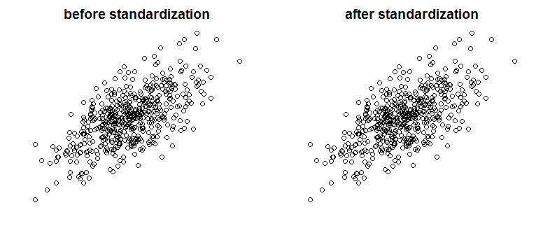
Can you spot the difference? As you can see, I purposefully removed the axis labels, so to convince you that I'm not cheating, see the plots with added labels:
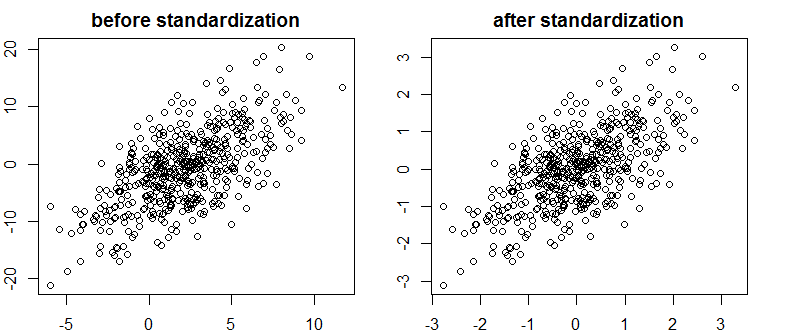
enter image description here

Mathematically speaking, if correlation is

$$ \newcommand{Corr}{\mathrm{Corr}} \newcommand{Cov}{\mathrm{Cov}} \Corr(X, Y) = \frac{\Cov(X,Y)}{\Var(X)\,\Var(Y)} $$

then with collinear variables we have

$$ \require{cancel} \begin{align} \Corr(X, Y) &= \frac{E[(X - \mu_X)(Y - \mu_Y)]}{\sigma_X\sigma_Y} \\ &=\frac{E[(X - \mu_X)(\cancel{\lambda_0} + \lambda_1 X - \cancel{\lambda_0} - \lambda_1\mu_X )]}{\sigma_X\;\lambda_1\sigma_X} \\ &= \frac{E[(X - \mu_X)(\lambda_1 X - \lambda_1\mu_X )]}{\sigma_X\;\lambda_1\sigma_X} \\ &= \frac{E[(X - \mu_X)\lambda_1( X - \mu_X )]}{\sigma_X\;\lambda_1\sigma_X} \\ &= \frac{\cancel{\lambda_1} E[(X - \mu_X)(X - \mu_X )]}{\sigma_X\;\cancel{\lambda_1}\sigma_X} \\ &= \frac{E[(X - \mu_X)(X - \mu_X )]}{\sigma_X\sigma_X} \end{align} $$

now since $\Cov(X,X) = \Var(X)$,

$$ \begin{align} &= \frac{\Cov(X, X)}{\sigma_X^2} = \frac{\Var(X)}{\Var(X)} = 1 \end{align} $$

While with standardized variables

$$ \begin{align} \Corr(Z_X, Z_Y) &= \frac{E[(Z_X - 0)(Z_Y - 0)]}{1 \times 1} \\ &= \Cov(Z_X, Z_Y) = \Var(Z_X) = 1 \end{align} $$

since $Z_X = Z_Y$...

Finally, notice that what Kruschke is talking about, is that standardizing of the variables makes life easier for the Gibbs sampler and leads to reducing of correlation between intercept and slope in the regression model he presents. He doesn't say that standardizing variables reduces collinearity between the variables.

$\endgroup$
0
$\begingroup$

Standardization does not affect the correlation between variables. They remain exactly the same. The correlation captures the synchronization of the direction of the variables. There is nothing in standardization that does change the direction of the variables.

If you want to eliminate multicollinearity between your variables, I suggest using Principal Component Analysis (PCA). As you know PCA is very effective in eliminating the multicollinearity problem. On the other hand PCA renders the combined variables (principal components P1, P2, etc...) rather opaque. A PCA model is always a lot more challenging to explain than a more traditional multivariate one.

$\endgroup$
2
  • $\begingroup$ A modern alternative, often better, is regularization. $\endgroup$ Commented Jul 16, 2019 at 10:02
  • $\begingroup$ I have tested variable selection between standard stepwise algorithms and LASSO. And, LASSO comes in a very distant second. LASSO penalizes variable influences, it can select weak variables over stronger variables. It can even cause variables signs to change. And, it breaks down the entire framework of statistical significance, Confidence Intervals, and Prediction Intervals. LASSO can at times work. But, look very carefully at the MSEs vs. Lambda graph and the Coefficients vs. Lambda graphs. That's where you can visually observe if your LASSO model worked. $\endgroup$
    – Sympa
    Commented Jul 19, 2019 at 4:55
0
$\begingroup$

It doesn't reduce the collinearity, it can reduce the VIF. Commonly we use VIF as indicator for concerns for collinearity.

Source: http://blog.minitab.com/blog/adventures-in-statistics-2/what-are-the-effects-of-multicollinearity-and-when-can-i-ignore-them

$\endgroup$
1
  • 2
    $\begingroup$ Welcome to the site. At present this is more of a comment than an answer. You could expand it, perhaps by giving a summary of the information at the link, or we can convert it into a comment for you. In addition, my reading of the linked post isn't quite that standardizing reduces the VIF without reducing collinearity. Their example is very specific & more nuanced than that. $\endgroup$ Commented Sep 19, 2018 at 1:16
0
$\begingroup$

This is actually a very important post because it refers to two crucial milestones in preprocessing and I would like to point out that the semantics of the word standardization are very heterogenous - while some may have a linear transformation in mind, others would refer to the workhorse scalers used in sklearn. This post made me reflect upon the implications of using the scalers.

This short exercise with the iris data from sklearn demonstates some of the above mentioned statements and adds another aspect:

  1. linear correlations do not change after a simple linear transformation by multiplication, or after scaling using linear scalers.
  2. VIF does not change after a simple multiplication by a constant, but it changes substantially if we apply scalers.
  3. linear correlations may change if we apply nonlinear scalers, like power transform.

The latter is very important because nonlinear change both i) VIF and ii) linear correlations. Therefore I would like to add that standardization may have implications for correlations if nonlinear scalers are applied. Sorry if the Python code below is clumsy, but I think that it is worth taking a closer look at the implications of scaling.

import math
from sklearn import preprocessing
import pandas as pd
from sklearn.datasets import load_iris
import copy as cp
from statsmodels.stats.outliers_influence import variance_inflation_factor

### VIF for original data
iris_data = load_iris()
iris_source = pd.DataFrame(data = iris_data['data'], columns = iris_data['feature_names'])
iris_cols = iris_source.columns.str.strip("(cm)")
iris_df = cp.deepcopy(iris_source)
iris_df.set_axis(iris_cols , axis=1,inplace=True)
vif_data = pd.DataFrame()
vif_data['Features'] = iris_df.columns
vif_data['VIF'] = [variance_inflation_factor(iris_df.values, i) for i in range(len(iris_df.columns))]
corrmat_orig = pd.DataFrame(round(iris_df.corr(), 4))

### Applying linear transformation by constant multiplication
iris_df_lintrans=cp.deepcopy(iris_df)
iris_df_lintrans['sepal length ']=iris_df['sepal length ']*10
iris_df_lintrans['sepal width ']=iris_df['sepal width ']*50
vif_data_lintrans = pd.DataFrame()
vif_data_lintrans['Features'] = iris_df_lintrans.columns
vif_data_lintrans['VIF'] = [variance_inflation_factor(iris_df_lintrans.values, i) for i in range(len(iris_df_lintrans.columns))]
corrmat_lintrans = pd.DataFrame(round(iris_df_lintrans.corr(), 4))

### Applying workhorse sklearn scalers, except nonlinear ones
from sklearn.preprocessing import StandardScaler, MinMaxScaler
scaler =  MinMaxScaler() ### can try MinMaxScaler or any other linear scaler
iris_scaler=scaler.fit(iris_df_lintrans)
iris_transformed=pd.DataFrame(iris_scaler.transform(iris_df_lintrans), columns=iris_df_lintrans.columns)
vif_data_scaled = pd.DataFrame()
vif_data_scaled['Features'] = iris_transformed.columns
vif_data_scaled['VIF'] = [variance_inflation_factor(iris_transformed.values, i) for i in range(len(iris_transformed.columns))]
vif_data_compare = pd.DataFrame()
vif_data_compare['Features'] = iris_transformed.columns
vif_data_compare['VIF_orig'] = vif_data['VIF']
vif_data_compare['VIF_lintrans'] = vif_data_lintrans['VIF']
vif_data_compare['VIF_scaled']= vif_data_scaled['VIF']
corrmat_scaled = pd.DataFrame(round(iris_transformed.corr(), 4))

### Print VIF for each case - VIF unachnged after multiplication but decreases after scaling using "workhorse" sklearn scalers
print('─' * 100) 
print(vif_data_compare)
print('─' * 100) 
### Print correlation matrix for each case - no changes
print(corrmat_orig)
print('─' * 100) 
print(corrmat_lintrans)
print('─' * 100) 
print(corrmat_scaled)
print('─' * 100) 

### Nonlinear scalers may distort linear correlations 

### Applying nonlinear PowerTransformer sklearn scaler
from sklearn.preprocessing import StandardScaler, MinMaxScaler, PowerTransformer
scaler =  PowerTransformer() ### can try MinMaxScaler or any other linear scaler
iris_scaler=scaler.fit(iris_df_lintrans)
iris_transformed=pd.DataFrame(iris_scaler.transform(iris_df_lintrans), columns=iris_df_lintrans.columns)
vif_data_scaled = pd.DataFrame()
vif_data_scaled['Features'] = iris_transformed.columns
vif_data_scaled['VIF'] = [variance_inflation_factor(iris_transformed.values, i) for i in range(len(iris_transformed.columns))]
vif_data_compare = pd.DataFrame()
vif_data_compare['Features'] = iris_transformed.columns
vif_data_compare['VIF_orig'] = vif_data['VIF']
vif_data_compare['VIF_lintrans'] = vif_data_lintrans['VIF']
vif_data_compare['VIF_scaled']= vif_data_scaled['VIF']
corrmat_scaled = pd.DataFrame(round(iris_transformed.corr(), 4))

print('─' * 100) 
print(corrmat_scaled)
print('─' * 100) 
$\endgroup$
-3
$\begingroup$

Standardization is a common way to reduce collinearity. (You should be able to verify very quickly that it works by trying it out on a couple of pairs of variables.) Whether you do it routinely depends on how much of a problem collinearity is in your analyses.

Edit: I see I was in error. What standardizing does do, though, is reduce collinearity with product terms (interaction terms).

$\endgroup$
4
  • $\begingroup$ Hmm, could you explain? Standardizing just changes the mean and variance of a random variable (to 0 and 1 respectively). This shouldn't change the correlation between two variables. I see how standardization can improve computational efficiency, but not how it reduces multicolinearity. $\endgroup$
    – Charlie
    Commented Oct 8, 2011 at 16:15
  • $\begingroup$ No, I;m lost ... how can that possibly change the linear dependence of the column elements in the matrix of predictors. (Isn't that what collinearity is about?) $\endgroup$
    – user6666
    Commented Oct 8, 2011 at 16:19
  • $\begingroup$ Although it is not correct that standardization changes collinearity in a purely mathematical sense, it can improve the numerical stability of algorithms to solve linear systems. That might be the source of the confusion in this reply. $\endgroup$
    – whuber
    Commented Oct 8, 2011 at 19:40
  • 1
    $\begingroup$ Standardization just does not reduce multicollinearity. It typically does not change the correlation between variables at all. $\endgroup$
    – Sympa
    Commented Oct 10, 2011 at 17:10

Your Answer

By clicking “Post Your Answer”, you agree to our terms of service and acknowledge you have read our privacy policy.