How to generate the posterior predictive distribution for hierarchal model in PYMC3

Question

See iPython notebook for full example

The below stochastic node y_pred enables me to generate the posterior predictive distribution:

with pm.Model() as model:
    alpha = pm.Gamma('alpha', alpha=.1, beta=.1)
    mu = pm.Gamma('mu', alpha=.1, beta=.1)
    y_pred = pm.NegativeBinomial('y_pred', mu=mu, alpha=alpha)
    y_est = pm.NegativeBinomial('y_est', mu=mu, alpha=alpha, observed=messages['time_delay_seconds'].values)

    start = pm.find_MAP()
    step = pm.Metropolis(start=start)
    trace = pm.sample(20000, step, start=start, progressbar=True)

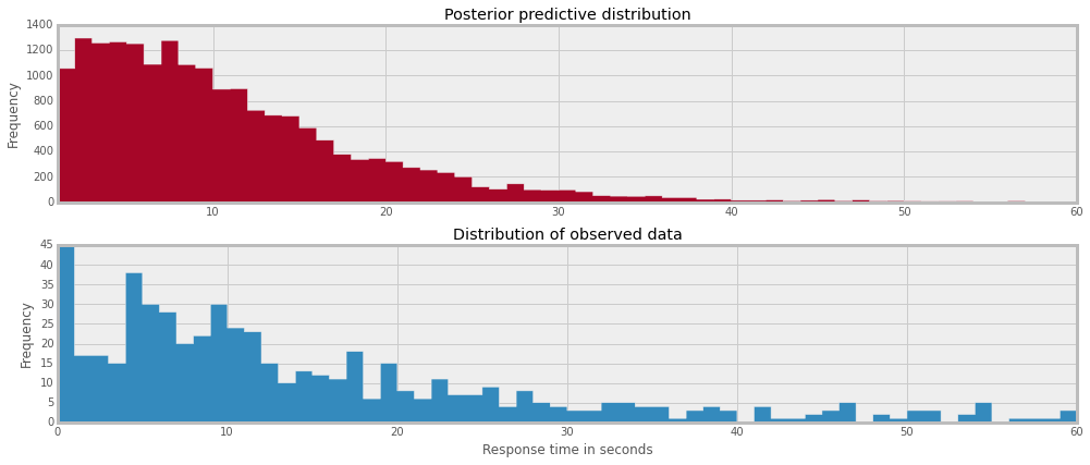
And the posterior predictive distribution plot:

Solution #1: @inversion points out that the shape parameter must be provided.

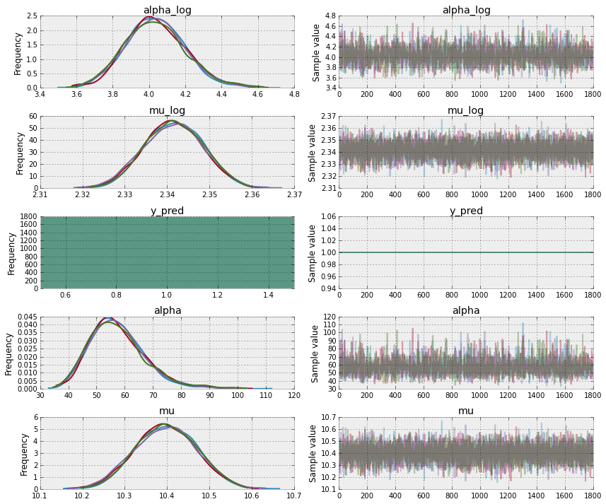
Problem #2: The samples from the posterior predictive are not correct. They get stuck at 0 or 1. Any ideas how to resolve this? I have only been able to reproduce this issue with hierarchal models.

See ipython notebook with issue reproduced.

Answer 1

The hierarchical model works if you specify the shape of y_pred.

y_pred = pm.NegativeBinomial('y_pred', 
                             mu=mu[people_idx], 
                             alpha=alpha[people_idx],
                             shape=people.shape)

Here's the trace:

And the posterior predictive plot (after the appropriate flattening):

y_pred = trace[burn::thin].get_values('y_pred').ravel()

You can, of course, use people_idx to compare posterior predictive plots of specific individuals.

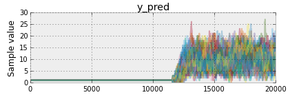
EDIT: Noting that y_pred takes a long time to snap out of a value of 1.

Answer 2

Second @inversion's answer. Note that there is (as of 5 minutes ago) proper support for drawing random samples directly from random variables. Here is an example of how to do this: http://pymc-devs.github.io/pymc3/posterior_predictive/