How to justify the error term in factorial ANOVA?

Question

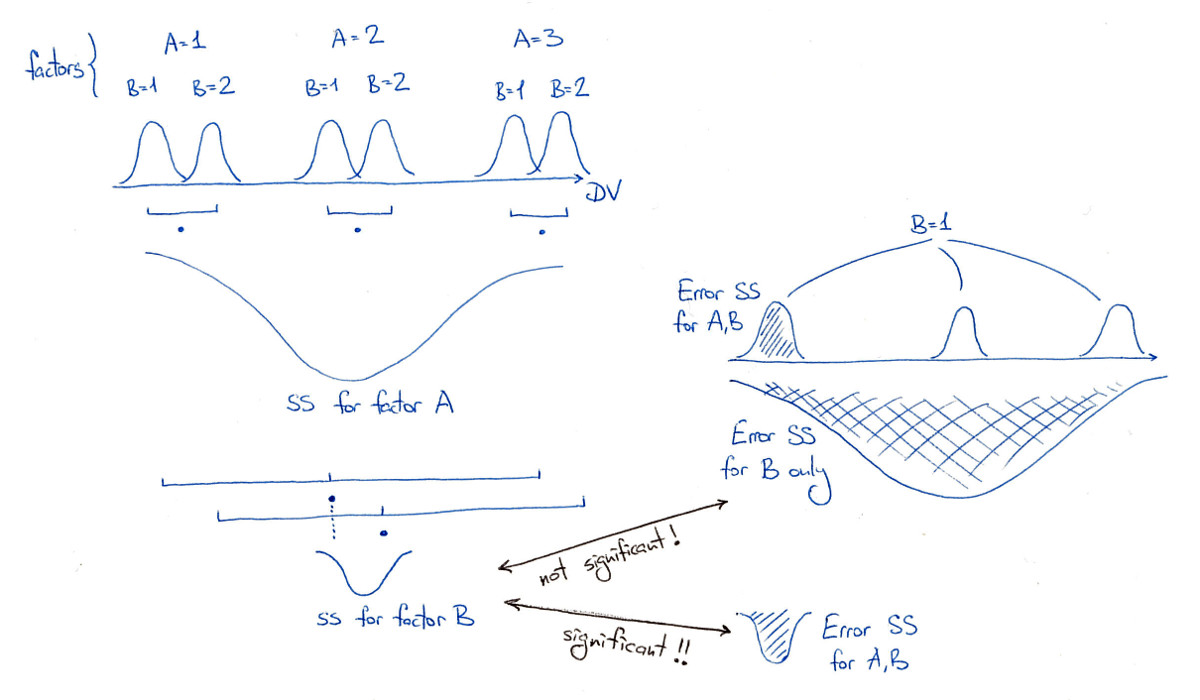
A probably very basic question about multi-factorial ANOVA. Assume a two-way design where we test both main effects A, B, and the interaction A:B. When testing the main effect for A with type I SS, the effect SS is calculated as the difference $RSS(1) - RSS(A)$, where $RSS(1)$ is the residual error sum of squares for the model with just the intercept, and $RSS(A)$ the RSS for the model with factor A added. My question concerns the choice for the error term:

How do you justify that the error term for this test is typically calculated from the RSS of the full model A + B + A:B that includes both main effects and the interaction? $$ F_{A} = \frac{(RSS_{1} - RSS_{A}) / (df_{RSS 1} - df_{RSS A})}{RSS_{A+B+A:B} / df_{RSS A+B+A:B}} $$

... as opposed to taking the error term from the unrestricted model from the actual comparison (RSS from just the main effect A in the above case): $$ F_{A} = \frac{(RSS_{1} - RSS_{A}) / (df_{RSS 1} - df_{RSS A})}{RSS_{A} / df_{RSS A}} $$

This makes a difference, as the error term from the full model is probably often (not always) smaller than the error term from the unrestricted model in the comparison. It seems that the choice for the error term is somewhat arbitrary, creating room for desired p-value changes just by adding/removing factors that aren't really of interest, but change the error term anyway.

In the following example, the F-value for A changes considerably depending on the choice for the full model, even though the actual comparison for the effect SS stays the same.

> DV  <- c(41,43,50, 51,43,53,54,46, 45,55,56,60,58,62,62,
+          56,47,45,46,49, 58,54,49,61,52,62, 59,55,68,63,
+          43,56,48,46,47, 59,46,58,54, 55,69,63,56,62,67)

> IV1 <- factor(rep(1:3, c(3+5+7, 5+6+4, 5+4+6)))
> IV2 <- factor(rep(rep(1:3, 3), c(3,5,7, 5,6,4, 5,4,6)))
> anova(lm(DV ~ IV1))                           # full model = unrestricted model (just A)
          Df  Sum Sq Mean Sq F value Pr(>F)
IV1        2  101.11  50.556  0.9342 0.4009
Residuals 42 2272.80  54.114

> anova(lm(DV ~ IV1 + IV2))                     # full model = A+B
          Df  Sum Sq Mean Sq F value   Pr(>F)    
IV1        2  101.11   50.56  1.9833   0.1509    
IV2        2 1253.19  626.59 24.5817 1.09e-07 ***
Residuals 40 1019.61   25.49                     

> anova(lm(DV ~ IV1 + IV2 + IV1:IV2))           # full model = A+B+A:B
          Df  Sum Sq Mean Sq F value    Pr(>F)    
IV1        2  101.11   50.56  1.8102    0.1782    
IV2        2 1253.19  626.59 22.4357 4.711e-07 ***
IV1:IV2    4   14.19    3.55  0.1270    0.9717    
Residuals 36 1005.42   27.93

The same question applies to type II SS, and in general to a general linear hypothesis, i.e., to a model comparison between a restricted and an unrestricted model within a full model. (For type III SS, the unrestricted model is always the full model, so the question doesn't arise there)

Answer 1

This is a very old question, and I believe that @gung's answer is very good (+1). But as it was not entirely convincing for @caracal, and as I don't fully follow all its intricacies either, I would like to provide a simple figure illustrating how I understand the issue.

---

Consider a two-way ANOVA (factor A has three levels, factor B has two levels) with both factors being obviously very significant:

SS for factor A is huge. SS for factor B is much smaller, but from the top figure it is clear that factor B is nevertheless very significant as well.

Error SS for the model containing both factors is represented by one of six Gaussians, and when comparing SS for factor B with this error SS, the test will conclude that factor B is significant.

Error SS for the model containing only factor B, however, is massive! Comparing SS for factor B with this massive error SS will definitely result in B appearing not significant. Which is clearly not the case.

That is why it makes sense to use error SS from the full model.

Answer 2

Update: To clarify some of the points I make in passing here, I have added some links to places where I discuss the relevant ideas more fully.

---

The F test checks if there is more variability (specifically mean squares) associated with a factor than there would be expected by chance. How much variation we might expect by chance is estimated from the sum of squared errors, that is, how much variability is due to (associated with) no known factor. These are your residuals, what is left over after having accounted for everything you know about. In your example, $RSS_{A}$ contains more than just the residual error, it also contains variability due to known factors. While the $SS_{A}$ are theorized to bounce around to some degree by chance, that amount is not theorized to be driven by the other known factors¹. Thus, it would be inappropriate to use $MS_{A}$ as the denominator in your F test. Moreover, using $MS_{A+B+A*B}$ gives you more power, decreasing the probability of type II error and shouldn't inflate type I error.

There are some further issues in your question. You mention that the $RSS_{full}$ is not always the lowest, and in your example, $MS_{A+B+A*B} > MS_{A+B}$. This is because the interaction is not actually associated with any variability of it's own. That $SS_{A*B} = 14.19$ appears to be due to nothing more than chance. There is a precise, but somewhat complicated, formula that specifies how power will change if different factors are included or excluded from the model. I don't have it at my fingertips, but the gist of it is simple: When you include another factor, the RSS decreases (giving you more power), but the $df_{R}$ goes down as well (yielding less power). The balance of this tradeoff is essentially determined by whether the SS associated with that factor are real, or only due to chance, which, in practice, is loosely indicated by whether the factor is significant². However, eliminating factors from the model that are not significant so as to get the right error term is logically equivalent to an automatic model search procedure, even if you don't have your software do it automatically for you. You should know that there are a lot of problems with doing this. Those problems, and alternative procedures are discussed elsewhere on CV³.

A final topic concerns the different types of SS. Firstly, the use of different types of SS doesn't not get you out of needing a logical justification of your analysis. But moreover, type I - III SS are related to a different issue. In your example, I gather your factors are orthogonal, i.e. you ran an experiment where you assigned equal n to each combination of factor levels. However, if you conduct an observational study, or if you have dropout issues, your factors will be correlated. The implications of that is that there is no unique way to partition the SS and so there's no unique answer for your analyses to produce. In other words, the various types of SS have to do with different possible numerators for your F test when your factors are correlated⁴.

<sub>1. Note that with multi-level models, a factor can be theorized to include variability from other factors, depending on how the model is specified. I am discussing ordinary ANOVA here, which is what you appear to be asking about.
2. See: How can adding a 2nd IV make the 1st IV significant?
3. See: Algorithms for automatic model selection.
4. See: How to interpret type I (sequential) ANOVA and MANOVA?</sub>

Answer 3

The justification is that factor A is explaining a larger percent of the unexplained variation in the A+B model compared to the A model, since factor B explains a significant portion (and thus 'removes' it from the analysis).