It's hard to step in when you had people commenting of the caliber of the names above, but I did tried to understand this the silly way... Using the power of [R] to simulate mathematical problems. So I hope it sheds some light into what these uncertainty quantifications attached to the regression parameters mean - that was the question...
So from the perspective of the frequentist there is this Platonic world of absolute representation of every single individual - the population, and we are looking at the shadows on the wall of the cave - the sample. We know that no matter how much we try we'll be off, but we want to have an idea of how far we'll be from the truth.
We can play god, and pretend to create the population, where everything is perfect, and the parameters governing the relationships between variables are glimmering gold. Let's do that by establishing that the variable $x$ will be related to the variable $y$ through the equation, $y = 10 + 0.4\,x$. We define the x's as x = seq(from = 0.0001, to = 100, by = 0.0001 (that is $1 \,million$ observations). The y's will therefore be calculated as y <- 0.4 * x + 10. We can combine these values in a data.frame: population = data.frame(x, y).
From this population we will take $100$ samples. For each sample, we will randomly select $100$ rows of data from the dataset. Let's define the function for sampling rows:
sam <- function(){
  s <- population[sample(nrow(population),100),]
  s$y <- s$y + rnorm(100, 0, 10)
  s
}
Notice that we are no longer in paradise - now we have noise (rnorm).
And we are going to collect both the intercepts and the slopes (I'll call them betas) of the OLS linear regression run on each one of these $100$ samples. Let's write some lines of code for this:
betas <- 0
intercepts <- 0
for(i in 1:100){
  s <- sam()
  fit <- lm(y ~ x, data = s)
  betas[i] <- coef(fit)[2]
  intercepts[i] <- coef(fit)[1]
}
And combine both into a new data.frame: reg_lines <- data.frame(intercepts, betas). As expected given the normal randomness of the noise the histogram of the slopes will be gaussian looking:

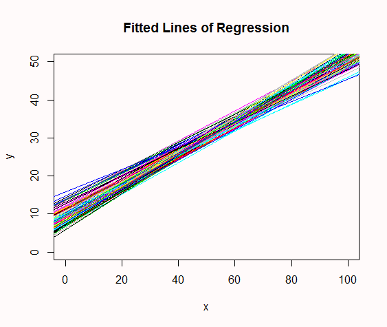
And if we plot all the regression lines that we fitted in each single one of the $100$ samples from the rows in the population we'll see how any single one is just an approximation, because they do oscillate between a maximum and a minimum in both intercept and slope. This is what they look like:

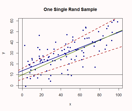
But we do live in the real world, and what we have is just a sample... Just one of those multicolored lines, through which we are trying to estimate the truth (i.e. intercept of $10$ and slope of $0.4$). Let's conjure this sample: S <- population[sample(nrow(population), 100),]; S$y <- S$y + rnorm(100, 0, 10), and its OLS regression line: fit <- lm(y ~ x, data = S).
Since we are playing god, let's plot our biased sample (dark blue dots of the with dark blue fitted regression line) together with the true line in solid green, and the maximum and minimum combinations of intercepts and slopes we got in our simulation (dashed red lines), giving us an idea of how off we could possibly be from the true line):

Let's quantify this possible error using a Wald interval for the slopes to generate the 5% confidence interval:
coef(fit)[2] + c(-1,1) * 1.96 * summary(fit)$coefficients[4], where summary(fit)$coefficients[4] is the calculated standard error of the estimated slope. This gives us; 0.2836088 to 0.4311044 (remember the "true" value $0.4$).
And for the intercept: coef(fit)[1] + c(-1,1) * 1.96 * summary(fit)$coefficients[3], which give us: 9.968347 to 17.640500.
Finally, let's compare these values by those generated by [R] when we type:
confint(fit)
(Intercept) 9.9204599 17.688387
x           0.2826881  0.432025
Pretty close...
OK, so this is a very intuitive approach at seeing what the confidence intervals are trying to answer. And as for the $p$-values, you can read how they are generated here. In general, the text notes that if the regression coefficient in the population is $0$ ($H_o: \beta = 0$) the $t$-statistic will be:
$$t = \frac{\hat\beta_{yx}-\beta{yz}}{SE_{\hat\beta}}= \frac{\hat\beta_{yx}}{SE_{\hat\beta}}$$.
The $SE_{\hat\beta}$ (which we used in the Wald interval) can be calculated in different ways, although the formula given in the text quoted is:
$SE_{\hat\beta}=\sqrt{\frac{var(e)}{var(x) \, (N-2)}}$. If we calculate this manually:
The variance of the independent variable for our sample is: var_x <- (sd(S$x))^2 = 719.0691. The variance for the errors is: var_e <- sum((residuals(fit)- mean(residuals(fit)))^2)/(nrow(S)-1) = 99.76605. And N - 2 = 98 (we lose one $df$ both for the intercept and the slope). Hence, $SE_{\hat\beta} = \small 0.03762643$ ((SE <- sqrt(var_e/(var_x * (N - 2))))). Which happily coincides with that obtained for the slope of x by [R]:
summary(fit)
Coefficients:
            Estimate Std. Error t value Pr(>|t|)
(Intercept) 13.80442    1.95718   7.053 2.49e-10 ***
x            0.35736    0.03763   9.497 1.49e-15 ***
So $t=\frac{\hat\beta_{yx}}{SE_{\hat\beta}}= \small 0.3573566 / 0.03762643=9.497488 $ ((t <- coef(fit)[2]/SE)). What else? Right, the $p$-value... pt(9.497488, 98, lower.tail = F) = 7.460233e-16 ~ 0.


