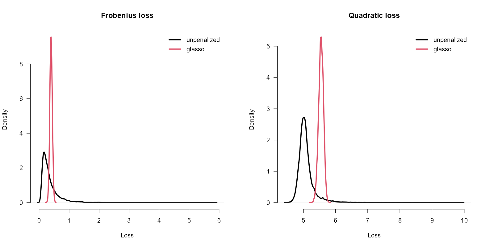
The short answer is that you should not in general expect improvements in estimated partial correlations when applying a non-zero amount of shrinkage when $n > p$.
The purpose of glasso
Least absolute shrinkage and selection operator (LASSO), and so also the graphical LASSO, applies $\ell_1$-norm regularized estimation, such that smaller estimates are shrunk to zero, leaving 'selected' non-zero estimates. Choosing $\lambda > 0$ implicitly incorporates prior information about the sparsity of $\mathbf{\Theta}$, but it does not provide any information about which elements should be shrunk to zero. All elements of $\mathbf{\Theta}$ will be shrunk.
Even for as little as $p=7$ variables like in the example provided, there are as many as $p(p-1)/2=21$ partial correlations that can be computed, so the prospect of a method that can select the non-zero ones is appealing. However, this is only one of three major purposes that glasso provides:
- Sparseness: Off-diagonal elements of $\mathbf\Theta$ are shrunk to zero;
- Invertability: When $n < p$, the empirical covariance matrix $\mathbf{S} = \hat{\mathbf\Sigma}^{-1}$ is singular and $\hat{\mathbf\Theta}$ cannot be obtained by inverting $\mathbf{S}$. Any amount of shrinkage $\lambda>0$ guarantees $\mathbf{S}$ is invertible;
- Speed: Inverting a matrix is a very costly operation for large $p$. The (imposed) sparseness of $\mathbf\Theta$ can be exploited using a block-coordinate descent approach. This is what the original paper on glasso by Friedman, Hastie & Tibshirani (2008) uses and it leads to several orders of magnitude improvement.
In the example provided in the question, none of these three appear to be of primary interest. Instead, the actual magnitude of the partial correlations matters most, and since $n>p$, this can simply be achieved by inverting $\mathbf{S}$. That does leave the question of how to identify the important/non-zero elements of $\hat{\mathbf\Theta}$. Fortunately, there are alternatives to glasso for this.
Sparse $\hat{\mathbf\Theta}$ without glasso
For glasso, the estimation and sparsification of the precision matrix $\mathbf\Theta$ are one and the same. This question is a great example where it is desirable to separate the estimation and selection. Since in the example $n\gg p$, this could be achieved by simply inverting the empirical covariance matrix $$\hat{\mathbf\Theta} = \hat{\mathbf\Sigma}^{-1},$$ and thresholding the resulting precision matrix. If you know a priori how many elements should be non-zero, you can simply pick the top $k$ absolute off-diagonal elements. The only remaining step is to convert precision to partial correlation: $$\rho_{ij} = \frac{-\hat{\theta}_{ij}}{\sqrt{\theta_{ii} \theta_{jj}}}$$
In absence of prior information on the number of non-zero elements, an elegant way to induce sparseness is by using a local false discovery rate (Efron, 2007). An implementation for this approach is available in the sparsify function of the rags2ridges package. In cases where $n < p$, a ridge-penalized inverse covariance matrix could be estimated, which is what the rags2ridges package was made for (Peeters, Bilgrau & van Wieringen 2022).
Comparing glasso and unpenalized estimation when $n \gg p$
To add some weight to the claims made in this post, here is an experiment using the same parameters as the simulation mentioned in the question. For this, we need to randomly simulate sparse $\mathbf\Theta$s, for which we can use the suggestion in this post. We also need a loss function to determine the error between $\mathbf\Theta$ and $\hat{\mathbf\Theta}$, for which we can use the squared Frobenius loss, or the quadratic loss, as implemented in rags2ridges.
require("glasso")
require("rags2ridges") # For Frobenius loss

# From: https://stats.stackexchange.com/a/587914/176202
# Create a sparse orthogonal matrix using `n` right multiplications by
# 2 X 2 rotation matrices.
#
rQ <- function(d, n = 0) {
  alpha <- runif(n, 0, 2 * pi)  # Rotation angles
  #
  # Generate random rotation planes.
  #
  i <- sample.int(d, n, replace = TRUE)
  j <- (sample.int(d - 1, n, replace = TRUE) + i - 1) %% d + 1
  #
  # Create the result through sequential right multiplication.
  #
  Q <- diag(1, d, d)
  for (k in seq_len(n)) {
    IJ <- c(i[k], j[k])
    c. <- cos(alpha[k])
    s. <- sin(alpha[k])
    Q[, IJ] <- Q[, IJ] %*% matrix(c(c., s., -s., c.), 2)
  }
  return(Q)
}

set.seed(2024)
p       <- 7
nonzero <- 6
lambda  <- 1:p                      # Eigenvalues of the covariance matrix
Q       <- rQ(p, nonzero - 1)       # A random sparse orthogonal matrix
Theta   <- crossprod(Q, Q / lambda) # The true precision matrix
Sigma   <- solve(Theta)
L       <- chol(Sigma)

MC <- 1e4
Theta_unpenalized <- vector(mode = "list", length = MC)
Theta_lasso       <- vector(mode = "list", length = MC)
for(i in 1:MC){
  n <- 50
  Z <- matrix(rnorm(n * p), nrow = n, ncol = p)
  X <- Z %*% L
  S <- cov(X)
  Theta_unpenalized[[i]] <- solve(S)
  x                      <- glasso(S, rho = exp(-1/2))$wi
  x[lower.tri(x)]        <- t(x)[lower.tri(x)]
  Theta_lasso[[i]]       <- x
}
Floss_unpenalized <- sapply(Theta_unpenalized, function(E){
  loss(E, Theta, type = "frobenius")
})
Floss_lasso <- sapply(Theta_lasso, function(E){
  loss(E, Theta, type = "frobenius")
})
Qloss_unpenalized <- sapply(Theta_unpenalized, function(E){
  loss(E, Sigma, type = "quadratic")
})
Qloss_lasso <- sapply(Theta_lasso, function(E){
  loss(E, Sigma, type = "quadratic")
})
d_F_u <- density(Floss_unpenalized)
d_F_l <- density(Floss_lasso)
d_Q_u <- density(Qloss_unpenalized)
d_Q_l <- density(Qloss_lasso)
par(mfrow = c(1, 2))
plot(d_F_u, main = "Frobenius loss", xlab = "Loss",
 bty = "n", las = 1, lwd = 3,
 xlim = range(c(d_F_u$x, d_F_l$x)),
 ylim = range(c(d_F_u$y, d_F_l$y)))
lines(d_F_l, col = 2, lwd = 3)
legend("topright", c("unpenalized", "glasso"),
   lwd = 3, col = 1:2, bty = "n")
plot(d_Q_u, main = "Quadratic loss", xlab = "Loss",
 bty = "n", las = 1, lwd = 3,
 xlim = range(c(d_Q_u$x, d_Q_l$x)),
 ylim = range(c(d_Q_u$y, d_Q_l$y)))
lines(d_Q_l, col = 2, lwd = 3)
legend("topright", c("unpenalized", "glasso"),
       lwd = 3, col = 1:2, bty = "n")
par(mfrow = c(1, 1))
(Note that the forced symmetry in the code for glasso is required due to an asymmetry in the glasso solution pointed out in Rolfs & Rajaratnum (2013).)

From the picture, it is evident that the unpenalized inverse covariance matrix estimation outperforms the glasso (using $\lambda = e^{\frac{1}{2}}$, which on average results in more or less 6 non-zero elements). Interestingly, it also shows what we expect in general from regularized estimation: Reduced variance at the cost of bias.
Efron, B. (2007). Size, power and false discovery rates. The Annals of Statistics, 35(4), 1351–1377. https://doi.org/10.1214/009053606000001460
Friedman, J., Hastie, T., & Tibshirani, R. (2008). Sparse inverse covariance estimation with the graphical lasso. Biostatistics (Oxford, England), 9(3), 432–441. https://doi.org/10.1093/biostatistics/kxm045
Rolfs, B. T., & Rajaratnam, B. (2013). A note on the lack of symmetry in the graphical lasso. Computational Statistics & Data Analysis, 57(1), 429–434. https://doi.org/10.1016/j.csda.2012.07.013
Peeters, C. F. W., Bilgrau, A. E., & van Wieringen, W. N. (2022). rags2ridges: A One-Stop-ℓ2-Shop for Graphical Modeling of High-Dimensional Precision Matrices. Journal of Statistical Software, 102(4), 1–32. https://doi.org/10.18637/jss.v102.i04

