8
$\begingroup$

I've run a fully within-subjects repeated-measures ANOVA using the aov() function. My dependent variable is not normally distributed, so I'm very interested in running assumption tests on my analysis. It seems that just calling plot() on the output doesn't work for repeated-measures, so I've manually taken the residuals and the fitted values for a model of interest, and have plotted them against each other. I'm assuming that this is how I would plot to test for the assumption of Homoskedasticity.

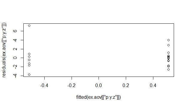
The plot comes out with 2 vertical bands (please see the image below). It turns out the fitted values are all centred around 2 values (although according to == they are not exactly equal), where one is the negative of the other.

I have 2 questions:

1) Is this the correct way to manually test the assumption homoskedasticity? If not, how would I go about it from repeated-measures designs (since just calling plot() doesn't work)?

2) If it is correct, what is this plot telling me? Why are the fitted values so clustered? What can I conclude from it?

Thanks heaps for any input here. Also, if you know of better ways to check (preferably plot) for assumptions in rm-ANOVAs, that would be useful information as well.

I've included some mock data here to replicate the scenario:

#Create mock data (there's probably a more efficient way to do this.. would also be nice to know! :) )
p <- sort(rep(1:20,8))
y <- rep(rep(1:2,4),20)
z <- rep(rep(c(1,1,2,2),2),20)
w <- rep(c(1,1,1,1,2,2,2,2),20)
x <- rnorm(160,10,2)

d <- data.frame(x,p=factor(p),y=factor(y),z=factor(z),w=factor(w))

#Run repeated-measures ANOVA
ex.aov <- aov(x ~ y*z*w + Error(p/(y*z*w)), d)

#Try to plot full object (doesn't work)
plot(ex.aov)

#Try to plot section of object (doesn't work)
plot(ex.aov[["p:y:z"]])

#Plot residuals against fitted (custom "skedasticity" plot - works)
plot(residuals(ex.aov[["p:y:z"]])~fitted(ex.aov[["p:y:z"]]))

enter image description here

Begin Edit

In light of the information provided by @Stefan , I've added some additional details below, using the improved data structure he proposed:

# Set seed to make it reproducible
set.seed(12)

#New variable names and generation
subj <- sort(factor(rep(1:20,8)))
x1 <- rep(c('A','B'),80)
x2 <- rep(c('A','B'),20,each=2)
x3 <- rep(c('A','B'),10, each=4)
outcome <- rnorm(80,10,2)

d3 <- data.frame(outcome,subj,x1,x2,x3)

#Repeated measures ANOVA
ex.aov <- aov(outcome ~ x1*x2*x3 + Error(subj/(x1*x2*x3)), d3)

#proj function
ex.aov.proj <- proj(ex.aov)

# Check for normality by using last error stratum
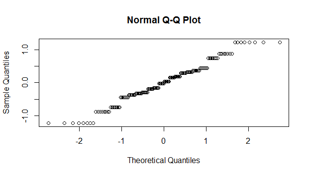
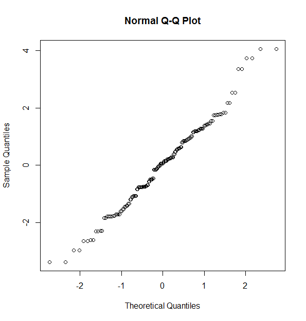
qqnorm(ex.aov.proj[[9]][, "Residuals"])
# Check for heteroscedasticity by using last error stratum
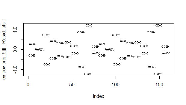
plot(ex.aov.proj[[9]][, "Residuals"])

The resulting plots are below:

Repeated measures normality check?

Repeated measures homoskedasticity check?

Can anyone interpret the images above (especially the last one)? It looks like there is clustering and pattern structure. Can it be used to infer the presence of heteroskedasticity?

$\endgroup$
3
  • $\begingroup$ "I'm assuming that this is how I would plot for "skedasticity" (sorry if I'm using the wrong term there)." .... what were your trying to achieve in plain English? $\endgroup$
    – Glen_b
    Commented Nov 23, 2015 at 7:33
  • $\begingroup$ @Glen_b Sorry for not being clear. I'm trying to run assumption checks on my analysis. My data (dependant variable) is not normally distributed, and I basically want to check whether this fact violates the assumption about normality of residuals, and/or the assumption about homoskedasticity. I'm afraid my statistical understanding of homoskedasticity isn't robust; I just know what it should look like when plotted, and that it is an assumption for a valid model. ...If I'm somehow barking up the wrong tree here it would be nice to know too... $\endgroup$
    – KerrBer
    Commented Nov 23, 2015 at 11:51
  • $\begingroup$ Thanks for the plot and the comment; they help. You could perhaps edit to include the information in your comment, which is useful. $\endgroup$
    – Glen_b
    Commented Nov 25, 2015 at 11:43

2 Answers 2

12
+200
$\begingroup$

I'm assuming that a model which was fitted using the Error() function within aov() won't work when using in plot() because you will get more than one error stratum from which you can choose. Now according to this information here, one should use the proj() function which will give you the residuals for each error stratum, which then can be used for diagnostic plots.

Edit 1 start

More information regarding multistratum models and the proj() function is given in Venables and Ripley, page 284 (but start from page 281): Residuals in multistratum analyses: Projections. In the second sentence they write (I highlighted in bold):

Thus fitted(oats.aov[[4]]) and resid(oats.aov[[4]]) are vectors of length 54 representing fitted values and residuals from the last stratum, based on 54 orthonormal linear functions of the original data vector. It is not possible to associate them uniquely with the plots of the original experiment. The function proj takes a fitted model object and finds the projections of the original data vector onto the subspaces defined by each line in the analysis of variance tables (including, for multistratum objects, the suppressed table with the grand mean only). The result is a list of matrices, one for each stratum, where the column names for each are the component names from the analysis of variance tables.

For your example that means:

ex.aov.proj <- proj(ex.aov)

# Check number of strata 
summary(ex.aov.proj)

# Check for normality by using last error stratum
qqnorm(ex.aov.proj[[9]][, "Residuals"])
# Check for heteroscedasticity by using last error stratum
plot(ex.aov.proj[[9]][, "Residuals"])

However, this will also lead into plots which I cannot fully interpret (especially the second one).

In their case, the last stratum was the Within stratum. Since your model cannot estimate this (presumably due to your error term), I am not sure if simply using your last stratum is valid.

Hopefully someone else can clarify.

Edit 1 end

Edit 2 start

According to this source checking residuals to assess normality and heteroscedasticity should be performed without the Error() function.

In order to check assumptions, you need to not use the error term. You can add the term without error, but the F tests are wrong. Assumption checking is OK, however.

This seems reasonable to me but I hope someone else could clarify.

Edit 2 end

My alternative suggestion:

First, I changed your dataset slightly and set a seed to make it reproducible (might be handy for some problems you have in the future):

# Set seed to make it reproducible
set.seed(12)

# I changed the names of your variables to make them easier to remember
# I also deleted a few nested `rep()` commands. Have a look at the `each=` argument.
subj <- sort(factor(rep(1:20,8)))
x1 <- rep(c('A','B'),80)
x2 <- rep(c('A','B'),20,each=2)
x3 <- rep(c('A','B'),10, each=4)
outcome <- rnorm(80,10,2)

d3 <- data.frame(outcome,subj,x1,x2,x3)

Second, I used a linear mixed-effects model instead since you have repeated measures and hence a random term you can use:

require(lme4)
# I specified `subj` as random term to account for the repeated measurements on subject.
m.lmer<-lmer(outcome ~ x1*x2*x3 + (1|subj), data = d3)
summary(m.lmer)

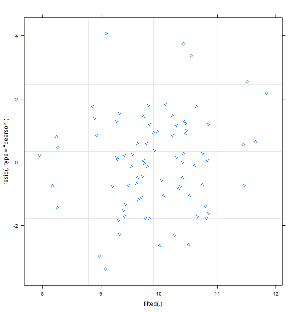
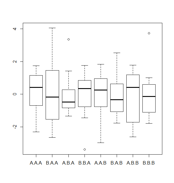
# Check for heteroscedasticity
plot(m.lmer)

enter image description here

# or
boxplot(residuals(m.lmer) ~ d3$x1 + d3$x2 + d3$x3)

enter image description here

# Check for normality
qqnorm(residuals(m.lmer))

enter image description here

Using the afex package you can also get the fixed effects in ANOVA table format (you can also use the Anova() function from the car package as another option):

require(afex)
mixed(outcome ~ x1*x2*x3 + (1|subj), data = d3, method="LRT")

Fitting 8 (g)lmer() models:
[........]
    Effect df    Chisq p.value
1       x1  1     0.04     .84
2       x2  1     2.53     .11
3       x3  1  7.68 **    .006
4    x1:x2  1  8.34 **    .004
5    x1:x3  1 10.51 **    .001
6    x2:x3  1     0.31     .58
7 x1:x2:x3  1     0.12     .73

Check ?mixed for the various options you can choose. Also regarding mixed models, there is a lot of information here on Cross Validated.

$\endgroup$
16
  • $\begingroup$ Wow, I had no idea about the integer-to-factor issue. This changes the structure of the output, but will this change the results as well (a quick test suggests that it does, but I want to be sure)? This is important in my case because: 1) I load my data in from MATLAB, meaning it is loaded as a dataframe with numeric variables. Is there a way to convert these variables to factors post-hoc that will avoid the aov() issue? 2) I have cross-validated my results with a repeated-measures ANOVA in SPSS, and get the same results. If the integer-to-factor issue changes the results, this is strange. $\endgroup$
    – KerrBer
    Commented Dec 7, 2015 at 11:38
  • 1
    $\begingroup$ @Stefan can you provide additional information about factor in aov? $\endgroup$
    – Tim
    Commented Dec 7, 2015 at 16:36
  • 1
    $\begingroup$ @Stefan I'd also appreciate some clarification on the issues with factor in aov. Although your examples work, I just tried to apply your suggestion to my data, and it didn't change anything. Explicitly, I applied the following to my numeric variables within a dataframe (2 examples below): results$Inversion <- as.character(results$Inversion) results$Inversion <- factor(results$Inversion, levels=c(0,1,2), labels=c("control", "upright", "inverted")) results$ID <- as.character(results$ID) results$ID <- factor(results$ID, levels=c(101:131), labels=as.character(1:31)) $\endgroup$
    – KerrBer
    Commented Dec 7, 2015 at 17:02
  • 1
    $\begingroup$ @Stefan so basically, the difference between ex.aov0 and ex.aov1 is that in the first case you treat p as factor, so as a dummy variable and in the second case you treat p as continuous variable. So aov works fine, there is no bug and it was your coding mistake. Please edit your answer to remove the misleading part about "bug" in aov since there is no bug and it does not make any change if you are using integers transformed to factors or character vector transformed to factors. $\endgroup$
    – Tim
    Commented Dec 7, 2015 at 18:35
  • 1
    $\begingroup$ @KerrBer, I prepared another plot that helps to better understand the pattern that we see but I don't understand how these residuals were calculated... There is a another link I found that says In order to check assumptions, you need to not use the error term.. I will add this to my answer and maybe someone else can explain. $\endgroup$
    – Stefan
    Commented Dec 11, 2015 at 2:06
0
$\begingroup$

Full disclaimer: I love using R for many different analyses, but I do not like doing ANOVAs in R.

Question 1: In the analytic context of ANOVAs, I'm more familiar with evaluating this assumption via tests of homogeneity of variances, vs. plotting homo/heteroscedasticity and visually evaluating it. Though there are multiple tests of homogeneity of variance, the one I see the most is Levene's test. In R , it appears you can do this via the car package using the leveneTest function.

Based on your data it would look like this: leveneTest(x ~ y*z*w, d). Note, that I don't think you are able to specify the repeated-measures error structure in this function, and in all honesty, I'm not sure if/to what extent that matters for Levene's test. Comparing with other stastical analysis software, it seems that there is some variability in terms of how Levene's test in repeated-measures ANOVA is carried out. SPSS, for example, provides separate between-group Levene's tests for each level of your repeated-measure, whereas the leveneTest function provides a comprehensive test of all levels of all variables--other software might have alternative approaches too. Anyways, the SPSS approach also seems to ignore the dependency of the data by only evaluating the between-group homogeneity of variance.

Question 2: If you're going to use a test of homogeneity of variance--Levene's or otherwise--it would probably be more informative to create simple bar-plots of the variances by each level of your variables (because that is what your homogeneity of variance test is explicitly evaluating). You could do this easily by estimating the variance of your outcome for every combination of your variables' levels, and then plotting them in base R, or using the ggplot2 package.

$\endgroup$
2
  • 3
    $\begingroup$ On a contrary note: I have (repeatedly) advised here against explicitly testing the assumption. $\endgroup$
    – Glen_b
    Commented Dec 6, 2015 at 7:41
  • 1
    $\begingroup$ @Glen_b can you link to a rationale for why? $\endgroup$
    – jsakaluk
    Commented Dec 6, 2015 at 13:31

Your Answer

By clicking “Post Your Answer”, you agree to our terms of service and acknowledge you have read our privacy policy.

Not the answer you're looking for? Browse other questions tagged or ask your own question.