Issues with Importance sampling for flat prior

Question

I am trying to draw Bayesian inference via importance sampling for a parameter $\xi$ attached with an (unbounded) flat prior. This seems problematic as this is clearly not a probability measure but rather a measure with mass infinity. Under a $t$-distributed likelihood with known $\sigma^2 $ and $\nu$ I obtain $$\log \mathcal{L}(y|\xi)=\frac{-\nu-1}{2}\sum_{t=1}^{T}\log\left(1+\frac{(y_t-\xi)^2}{\nu\sigma^2}\right)$$

Is this the kernel of a known probability distribution in $\xi_i$?

As I doubt so, I am searching for a importance density that helps me computing sensible weights. For example, if I chose $\xi_i \sim N(\mu,\sigma_\xi ^2)$ as importance density, my weights will look like $$w_i=\exp\left(\log\{\mathcal{L}(y|\xi_i)\}+\frac{1}{2\sigma_\xi ^2}(\xi_i-\mu)^2\right).$$ Simulating gives me an extremely high number of weights being equal to $0$.

How can I overcome this problem?

**Remark: I updated the notation due to a mistake. **

Answer 1

Preliminary: the issue has nothing to do with using a flat prior. A regular prior would lead to a non-standard posterior all the same.

This model means that you observe $T$ random variates from a $t$ distribution with $\nu$ degrees of freedom and use a Gaussian as your importance proposal. This makes complete sense as the posterior on $\xi$, while non-standard, is quite close to a Gaussian. While the exact posterior variance of $\xi$ is unknown, it should be close to $s^2/T$, the empirical variance of the data divided by the sample size. I suggest using $\bar{y}_n$ for $\mu$ and $100 s^2/T$ for $\sigma^2_\xi$ in order to ensure wide enough simulations. (This can be calibrated by looking at the likelihood values. For instance, use plot(prop,like(prop)) to observed if the likelihood goes up and then down again. I started with a factor of 4 and this was too small.)

With such a proposal, here is an R code that runs the said importance sampling experiment, with no visible difficulty:

n=35 #your T
T=1e5 #my importance sample size
deg=3 #nu
data=rt(n,df=deg)
like=function(the){
  if (length(the)>1){
   ou=rep(0,length(the))
   for (i in 1:length(the))
    ou[i]=sum(dt(data-the[i],df=deg,log=TRUE))
  }else{
  ou=sum(dt(data-the,df=deg,log=TRUE))}
  return(ou)}
prop=rnorm(T,mean=mean(data),sd=10*sd(data)/n)
iw=like(prop)-dnorm(prop,mean=mean(data),sd=10*sd(data)/n,log=TRUE)
iw=exp(iw-max(iw))

For instance, here is the range of the importance weights:

> range(iw)
[1] 0.0003463474 1.0000000000

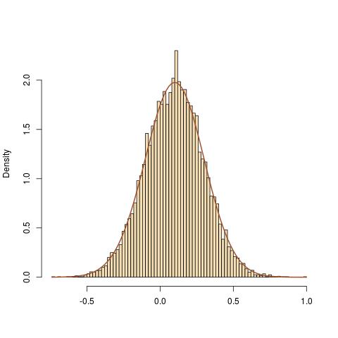
And here is the fit between the weighted histogram and the normalised target posterior density.