Bayesian inference on X's parameters by X's boundary sample data

Question

Given $R = \{r_1,r_2,....\}$ and $T = \{t_1,t_2,....\}$ where $R < X < R+T$.

If $X$'s distribution function $F(x,\alpha, \beta)$ is known.

To estimate parameters $\alpha$ and $\beta$, I want to use following equation.

$p(\alpha, \beta|r<X<t) = p(\alpha, \beta)p(r<X<t|\alpha, \beta)$ where the parameter's can be assume to be Uniformly distributed as prior. And the posterior probability is updated by likelihood function with sample $r_n$ and $t_n$.

Is this correct application of bayesian inference?

Answer 1

Yes, that should be fine. As a detail, note that the relation should be of proportionality, not equality. That is, \begin{equation*} p(\alpha, \beta \, | \, r < X < r + t) \propto p(\alpha, \beta) p(r < X < r + t \, | \, \alpha, \beta). \end{equation*}

You can use $F(x, \alpha, \beta)$ to calculate $p(r < X < r + t \, | \, \alpha, \beta)$ by way of $F(r + t, \alpha, \beta) - F(r, \alpha, \beta)$ - assuming $F$ is the cumulative distribution function as per the standard notation.

To help see that this is valid you can think of a Bernoulli random variable $Y_{r, t}$, where $Y_{r, t} = 1$ if $X$ is in the interval $(r, r+t)$ and is 0 otherwise. The standard Bernoulli probability is then described via $p(r < X < r + t)$, so you could rewrite your problem as \begin{equation*} p(\alpha, \beta \, | \, y_{r, t}) \propto p(\alpha, \beta) p(y_{r, t} \, | \, \alpha, \beta). \end{equation*}

As an example you can consider a simple model like this:

\begin{align*} \alpha, \beta & \sim \text{uniform(1, 10)} \\ X \, | \, \alpha, \beta & \sim \text{beta}(\alpha, \beta). \end{align*}

Here's some corresponding code (pardon the Haskell); note in particular that I've defined the likelihood in terms of boundary values:

logPrior l u a b
  | u < l = log 0
  | a < l || b < l || a > u || b > u = log 0
  | otherwise = log (density uniform a) + log (density uniform b) where
      uniform = uniformDistr l u

logLikelihood ps a b = foldl' (+) 0 (fmap (log . prob) ps) where
  beta = betaDistr a b
  prob (r, t)
    | r + t > 1 = 0
    | r < 0     = 0
    | otherwise = cumulative beta (r + t) - cumulative beta r

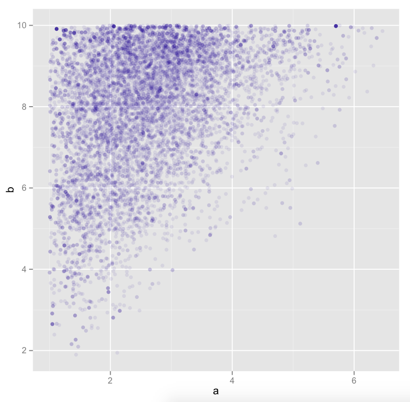
Here's the posterior, conditional on the observations

\begin{equation*} \{(r, t)\} = \{(0.1, 0.2), (0.08, 0.21), (0.1, 0.25), (0.09, 0.18)\} \end{equation*}

logPosterior [a, b]
  | a <= 0 || b <= 0 = log 0
  | otherwise        = logPrior 1 10 a b + logLikelihood obs a b where
      obs = [(0.1, 0.2), (0.08, 0.21), (0.1, 0.25), (0.09, 0.18)]

and we can collect some samples over the posterior parameter space via whatever method you have available (I've used a simple Metropolis sampler below):

For a different set of observations, say

\begin{equation*} \{(r, t)\} = \{(0.5, 0.2), (0.48, 0.21), (0.5, 0.25), (0.49, 0.18)\} \end{equation*}

you of course get a different posterior: