Combining individual terms from the predict() function

Question

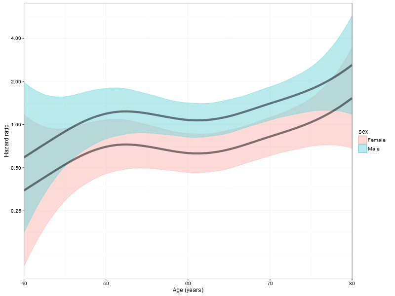
I want to merge several variables' estimate and also calculate the confidence intervals from the survival:::predict.coxph function's output. Just like the the predict.lm the function allows for estimating specific term estimates and sample errors for specific variables. The rms::contrast function has a function that allows contrasting one outcome with another and handles this very nicely, unfortunately under some circumstances I've found that I can't use the rm::contrast and it would be nice to use the predict function for estimating the same (or similar combined estimate). I'm particularly interested in this for survival functions as this becomes a must when a variable has a time-interaction estimate that needs to merge with the base estimate.

Adding variances

Getting the estimate is a simple sum exercise of the coefficient of interest:

$$\sum_{i=1}^{n}{est_i}$$

I originally thought that the variance could be calculated by

$$\sqrt{\sum_{i=1}^{n}{\hat{\sigma}_i^2}}$$

where $n$ is the number of terms. But as this doesn't really handle the complexity of predictor covariance, thus the formula should be:

$$Var(a*X + b*Y) = a^2*Var(X) + b^2*Var(X) + 2*a*b*Cov(X,Y)$$

This does make everything much more complicated, especially when one of the variances is a spline. I was hoping to use the predict function for getting the raw estimates and then merging them in some fashion:

library(survival)
library(magrittr)
library(dplyr)
data("lung", package = "survival")
lung$sex <- 
  factor(lung$sex,
         labels = c("Male", "Female"))
model <- coxph(Surv(time, status) ~ sex + pspline(age) + wt.loss, data=lung)

new_data <- data.frame(sex = rep(levels(lung$sex), each = 100),
                       age = rep(seq(40, 80, length.out = 100),
                                 times = 2),
                       wt.loss = median(lung$wt.loss, na.rm=TRUE))

m_pred <- predict(model,
                  newdata = new_data,
                  type = "terms",
                  terms = names(model$assign)[grep("sex|age", names(model$assign))],
                  se.fit = TRUE)

lapply(m_pred, function(x) knitr::kable(head(x), align = "r"))

This gives the result:

$fit


|       sex| pspline(age)|
|---------:|------------:|
| 0.2135748|   -0.7408014|
| 0.2135748|   -0.7064531|
| 0.2135748|   -0.6721696|
| 0.2135748|   -0.6379620|
| 0.2135748|   -0.6038413|
| 0.2135748|   -0.5698185|

$se.fit


|       sex| pspline(age)|
|---------:|------------:|
| 0.0705246|    0.6129619|
| 0.0705246|    0.5727195|
| 0.0705246|    0.5346473|
| 0.0705246|    0.4988786|
| 0.0705246|    0.4655234|
| 0.0705246|    0.4346488|

Here's what we get if we simply add these (Note: this is not the correct way):

new_data$fit <-
  rowSums(m_pred$fit)

new_data$se.fit <-
  apply(m_pred$se.fit, 1, function(x) x^2) %>% 
  colSums() %>% # apply flips the matrix, therefore the colSums
  sqrt()

library(ggplot2)
new_data %>% 
  mutate(risk = exp(fit),
         upper = exp(fit + 1.96*se.fit),
         lower = exp(fit - 1.96*se.fit)) %>% 
  ggplot(aes(y = risk, x = age, col = sex, fill = sex)) + 
  geom_ribbon(aes(ymax = upper, ymin = lower), alpha = .5) +
  scale_fill_hue(c=45, l=80) +
  scale_color_hue(c=45, l=80) +
  scale_y_log10(breaks=2^(-2:3)) +
  scale_x_continuous(expand = c(0,0)) +
  geom_line(lwd = 2, alpha = .5, color = "black") + 
  theme_bw() + 
  ylab("Hazard ratio") +
  xlab("Age (years)")

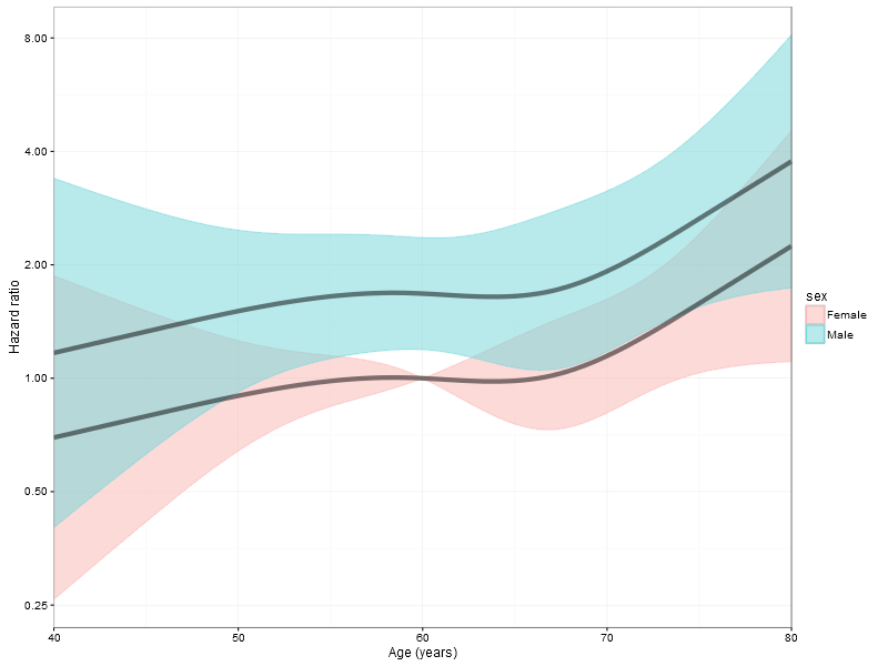
This plot is actually not that dissimilar from what I can get from the rms::contrast. It doesn't though have a waist and I'm uncertain of how to interpret the confidence interval, I guess they're the confidence interval for each individual estimated hazard ratio. Here's the rms version of above:

library(rms)
dd <- datadist(lung)
options(datadist = "dd")
# The pspline gives: Error in X[, mmcolnames, drop = FALSE] : subscript out of bounds
cph_model <- cph(Surv(time, status) ~ sex + rcs(age, 4) + wt.loss, data=lung)

# Now here's the contrast funciton in action
# We set the age to the age span of interest
# and then we specify that we're interested 
# in the two levels of the sex variable
# As reference we set the age to 60 and the 
# sex to female
cntr <- 
  contrast(cph_model,
           a = list(age = seq(40, 80, length.out = 100),
                    sex = levels(lung$sex)),
           b = list(sex = "Female",
                    age = 60))

# The contrast function returns a list that needs to be reformatted
# Note that the sex is interchanging while age is continuous
# - If you're unfamiliar with the coding I recommend extracting
#   one sex at the time and then merging them into one
data.frame(age = rep(seq(40, 80, length.out = 100), each = 2),
           sex = rep(levels(lung$sex), times = 100),
           risk = exp(cntr$Contrast),
           upper = exp(cntr$Upper),
           lower = exp(cntr$Lower)) %>% 
  ggplot(aes(y = risk, x = age, col = sex, fill = sex)) + 
  geom_ribbon(aes(ymax = upper, ymin = lower), alpha = .5) +
  scale_fill_hue(c=45, l=80) +
  scale_color_hue(c=45, l=80) +
  scale_y_log10(breaks=2^(-2:3)) +
  scale_x_continuous(expand = c(0,0)) +
  geom_line(lwd = 2, alpha = .5, color = "black") + 
  theme_bw() + 
  ylab("Hazard ratio") +
  xlab("Age (years)")

Gives the following plot:

My intuition so far on the subject

In my mind the variance combined from different estimates should only be a form of re-scaling, i.e. the variance is dependent on the unit and the unit can either be age in years or age in 20 years when comparing 40 years with 60 years. The 20 years age difference is simply a constant, i.e. I should multiply the variance by:

$$Var(c*\hat{\sigma}) = c^2 * Var(\hat{\sigma}^2) = 20^2 * Var(\hat{\sigma}^2)$$

The properties of the variance extends nicely to summing the variance between age and sex should be (b = 1):

$$Var(a*Age + b*Sex) = a^2*Var(Age) + Var(Sex) + 2*a*Cov(Age,Sex)$$

I understand that the key is in the variance-covariance matrix. Looking at the low covariance estimates between age and sex the similarity of the curves is not surprising:

>vcov(cph_model)
           sex=Female     age    age'   age'' wt.loss
sex=Female     0.0305  0.0004 -0.0006  0.0029   0e+00
age            0.0004  0.0013 -0.0024  0.0101   0e+00
age'          -0.0006 -0.0024  0.0054 -0.0250   0e+00
age''          0.0029  0.0101 -0.0250  0.1261  -1e-04
wt.loss        0.0000  0.0000  0.0000 -0.0001   0e+00

I guess that if my reasoning is correct it is rather straight forward to generate contrast from pure linear variables. As splines are inherently difficult to calculate by hand it seems that the predict with the terms attribute should provide a combined variance for age. Unfortunately I won't be able to get the covariance for the formula above between the two or can I get around this in some clever way?

By request

Here's the variance-covariance matrix for the first model:

> round(vcov(model), 4)
          sexFemale ps(age)3 ps(age)4 ps(age)5 ps(age)6 ps(age)7 ps(age)8 ps(age)9 ps(age)10 ps(age)11 ps(age)12 ps(age)13
sexFemale    0.0308  -0.0024  -0.0046  -0.0059  -0.0054  -0.0023  -0.0004  -0.0016   -0.0030   -0.0022    0.0002    0.0045
ps(age)3    -0.0024   0.5458   0.8321   0.9147   0.9022   0.8801   0.8734   0.8749    0.8764    0.8764    0.8760    0.8755
ps(age)4    -0.0046   0.8321   1.4123   1.5816   1.5576   1.5130   1.4993   1.5023    1.5053    1.5054    1.5047    1.5037
ps(age)5    -0.0059   0.9147   1.5816   1.8774   1.8551   1.7869   1.7640   1.7679    1.7728    1.7731    1.7723    1.7711
ps(age)6    -0.0054   0.9022   1.5576   1.8551   1.9087   1.8295   1.7910   1.7923    1.7988    1.7999    1.7993    1.7983
ps(age)7    -0.0023   0.8801   1.5130   1.7869   1.8295   1.8157   1.7658   1.7549    1.7594    1.7617    1.7622    1.7620
ps(age)8    -0.0004   0.8734   1.4993   1.7640   1.7910   1.7658   1.7743   1.7474    1.7394    1.7405    1.7423    1.7434
ps(age)9    -0.0016   0.8749   1.5023   1.7679   1.7923   1.7549   1.7474   1.7741    1.7497    1.7393    1.7389    1.7402
ps(age)10   -0.0030   0.8764   1.5053   1.7728   1.7988   1.7594   1.7394   1.7497    1.7783    1.7535    1.7394    1.7314
ps(age)11   -0.0022   0.8764   1.5054   1.7731   1.7999   1.7617   1.7405   1.7393    1.7535    1.7859    1.7620    1.7361
ps(age)12    0.0002   0.8760   1.5047   1.7723   1.7993   1.7622   1.7423   1.7389    1.7394    1.7620    1.8293    1.8429
ps(age)13    0.0045   0.8755   1.5037   1.7711   1.7983   1.7620   1.7434   1.7402    1.7314    1.7361    1.8429    2.0834
ps(age)14    0.0089   0.8750   1.5028   1.7699   1.7973   1.7618   1.7446   1.7415    1.7238    1.7102    1.8539    2.3164
wt.loss      0.0000  -0.0001  -0.0002  -0.0002  -0.0003  -0.0004  -0.0003  -0.0003   -0.0003   -0.0002   -0.0003   -0.0003
          ps(age)14 wt.loss
sexFemale    0.0089   0e+00
ps(age)3     0.8750  -1e-04
ps(age)4     1.5028  -2e-04
ps(age)5     1.7699  -2e-04
ps(age)6     1.7973  -3e-04
ps(age)7     1.7618  -4e-04
ps(age)8     1.7446  -3e-04
ps(age)9     1.7415  -3e-04
ps(age)10    1.7238  -3e-04
ps(age)11    1.7102  -2e-04
ps(age)12    1.8539  -3e-04
ps(age)13    2.3164  -3e-04
ps(age)14    3.0339  -3e-04
wt.loss     -0.0003   0e+00

As a minor note I commonly refer to log-hazard as hazard ratio, I know this is sloppy and I'm sorry for any confusion that it causes.

Trying to implement the $\delta$ method as suggested by AdamO.

From the comment I would interpret that I should:

$$Var(\delta hz = prediction_1 - prediction_2) = Var(prediction_1) * Var(prediction_2)*(logHazard(prediction_1) - logHazard(prediction_2))^2$$

This would be equivalent in R-code to:

m40_data <- 
  data.frame(sex = "Male",
             age = 40,
             wt.loss = median(lung$wt.loss, na.rm=TRUE))
f60_data <- 
  data.frame(sex = "Female",
             age = 60,
             wt.loss = median(lung$wt.loss, na.rm=TRUE))

pre_m40 <- 
  predict(cph_model, 
          newdata = m40_data, 
          se.fit = TRUE)
pre_f60 <- 
  predict(cph_model, 
          newdata = f60_data, 
          se.fit = TRUE)

log_hzrd <- 
  pre_m40$linear.predictors -
  pre_f60$linear.predictors
comb_se <- 
  sqrt(pre_m40$se.fit^2 * 
         pre_f60$se.fit^2 * 
         log_hzrd^2)

sprintf(
"Log Hazard: %.3f,
Combined s.e.: %.3f",
log_hzrd, comb_se) %>% cat

Gives:

Log Hazard: 0.155,
Combined s.e.: 0.010

If we compare this to the contrast function the variance is not even close:

cntr <- 
  contrast(cph_model,
           a = list(age = 40,
                    sex = "Male"),
           b = list(sex = "Female",
                    age = 60))
sprintf(
"Log Hazard: %.3f,
Combined s.e.: %.3f",
  cntr$Contrast, cntr$SE) %>% cat

Gives:

Log Hazard: 0.155,
Combined s.e.: 0.545

I guess I've misunderstood something in the instructions, looking at the Wikipedia page I realize that I need to somehow get this formula to work:

$$Var(h_r)=\sum_{i}{\left(\frac{\partial h_r}{\partial B_i}\right) Var(B_i) + \sum_{i}{\sum_{j \ne i}{\left(\frac{\partial h_r}{\partial B_i}\right)\left(\frac{\partial h_r}{\partial B_j}Cov(B_i,B_j)\right)}}}$$

While the formula looks complicated to an orthopaedic surgeon, I don't quite grasp the concept of the partial derivatives but it shouldn't be that complicated to convert into useful code. I guess the predict does this for the spline variables and the only covariances that actually are missing are the covariance of $Cov(age, sex)$ but this of course expands to $Cov(age_1,sex), Cov(age_2, sex), ...$ due to the spline.

Answer 1

Like a contrast, a hazard ratio is a ratio of instantaneous hazards, or a difference of log hazards. Unlike a contrast, the referent group, the denominator hazard, is fixed.

You can go one step further with this information. One can calculate a difference of hazard ratios (on the hazard ratio scale) using the delta method. I think most contrast implementations will give you this. Usually, you can tell this is the case because the contrast CIs are symmetric on the hazard ratio scale. Differences in hazard ratios are nonsensical to me. Differences in log hazard ratios become, themselves, hazard ratios between two groups of interest when exponentiated. This makes sense. When using contrast functionality, it's important to perform all calculations on the linear predictor scale before exponentiating the output.

The "bottleneck" in your plot is given by the referent group: i.e. women who are 50 years old. So the predicted hazard ratio for men who are 70 is a ratio of their predicted hazard over that of women who are 50 years old. This is completely different than the phenomenon attributed to the differences between confidence and prediction intervals.

Your predicted hazard ratio for 70 year old men would be interpreted as an interval in which, if the study were conducted an infinite number of times, would be expected to contain $100\times(1-\alpha)$% of other fitted hazard ratios. No matter how many times the study is redone, women who are 50 will always be the referent group, so their HR is always 1. That's why you observe the bottleneck in the plot. Therefore, there's no way to get rid of it.

I also note that your predicted hazard ratios are symmetric on the hazard ratio scale. I believe that you are not accounting for the fact that the covariance matrix applies to model effects on the linear predictor scale (log-hazard), and the fitted "hazard ratio" is exponentiated. To calculate asymptotically correct confidence intervals on the hazard ratio scale, you will need to apply the $\delta$-method, i.e.

$$\widehat{\log \left( \lambda_{t}(X_i)\right) - \log \left( \lambda_t(X_0) \right)} = \mathbf{X} \hat{\beta}$$

But the hazard ratio is given by:

$$\frac{\lambda_{t}(X_i)}{\lambda_{t}(X_0)} = \exp \left( \mathbf{X} \hat{\beta} \right)$$

You can easily apply the delta method to obtain what the approximate variance of the transformation of linear predictors is.

EDIT

On further inspection, I suspect the issue has to do with how pspline codes the continuous variable age. Can you show the output of pspline? I bet it standardizes the variable to some reasonable average or median value, so that age=50 becomes 0 and therefore a referent value.