Central limit theorem and the Pareto distribution

Question

Can somebody please provide a simple (lay person) explanation of the relationship between Pareto distributions and the Central Limit Theorem (e.g. does it apply? Why/ why not?)? I am trying to understand the following statement:

"the Central Limit Theorem doesn’t work with every distribution. This is due to one sneaky fact — sample means are clustered around the mean of the underlying distribution if it exists. But how can a distribution have no mean? Well, one common distribution that has no mean is the Pareto distribution. If you tried to calculate it using the usual methods, it would diverge to infinity."

Answer 1

The statement is not true in general -- the Pareto distribution does have a finite mean if its shape parameter ($\alpha$ at the link) is greater than 1.

When both the mean and the variance are finite ($\alpha>2$), the usual forms of the central limit theorem - e.g. classical, Lyapunov, Lindeberg will apply

See the description of the classical central limit theorem here

The quote is kind of weird, because the central limit theorem (in any of the mentioned forms) doesn't apply to the sample mean itself, but to a standardized mean (and if we try to apply it to something whose mean and variance are not finite we'd need to very carefully explain what we're actually talking about, since the numerator and denominator involve things which don't have finite limits).

Nevertheless (in spite of not quite being correctly expressed for talking about central limit theorems) it does have something of an underlying point -- if the shape parameter is small enough, the sample mean won't converge to the population mean (the weak law of large numbers doesn't hold, since the integral defining the mean is not finite).

---

As kjetil rightly points out in comments, if we're to avoid the rate of convergence being terrible (i.e. to be able to use it in practice), we need some kind of bound on "how far way"/"how quickly" the approximation kicks in. It's no use having an adequate approximation for $n> 10^{10^{100}}$ (say) if we want some practical use from a normal approximation.

The central limit theorem is about the destination but tells us nothing about how fast we get there; there are, however, results like the Berry-Esseen theorem theorem which do bound the rate (in a particular sense). In the case of Berry-Esseen, it bounds the largest distance between distribution function of the standardized mean and the standard normal cdf in terms of the third absolute moment, $E(|X|^3)$.

So in the case of the Pareto, if $\alpha\gt 3$, we can at least get some bound on just how bad the approximation might be at some $n$, and how quickly we're getting there. (On the other hand, bounding the difference in cdfs isn't necessarily an especially "practical" thing to bound -- what you're interested may not relate especially well to a bound on the difference in tail area). Nevertheless, it is something (and in at least some situations a cdf bound is more directly useful).

Answer 2

I will add an answer showing how bad the approximation from the central limit theorem (CLT) can be for the Pareto distribution, even in a case where the assumptions for CLT is fulfilled. The assumption is that there must be a finite variance, which for the Pareto means that $\alpha > 2$. For a more theoretical discussion of why this is so, see my answer here: What is the difference between finite and infinite variance

I will simulate data from the Pareto distribution with parameter $\alpha=2.1$, so that the variance "just barely exists". Redo my simulations with $\alpha=3.1$ to see the difference! Here is some R code:

###  Pareto dist and the central limit theorem
###
require(actuar) # for (dpqr)pareto1()
require(MASS) #  for Scott()
require(scales) # for alpha()
# We use (dpqr)pareto1(x,alpha,1)
#
alpha <- 2.1  #  variance just barely exist
E <-  function(alpha) ifelse(alpha <= 1,Inf,alpha/(alpha-1))
VAR <- function(alpha) ifelse(alpha <= 2, Inf, 
        alpha/((alpha-1)^2 * (alpha-2)))

R <- 10000
e <-  E(alpha)
sigma  <-  sqrt(VAR(alpha))
sim <-  function(n) {
    replicate(R, {x <- rpareto1(n,alpha,1)
        x <- x-e
        mean(x)*sqrt(n)/sigma },simplify=TRUE)
}
sim1 <- sim(10)
sim2 <- sim(100)
sim3 <- sim(1000)
sim4 <- sim(10000) # do take some time ...

### These are standardized so have all 
### theoretically variance 1.
### But due to the long tail, the empirical variances are 
### (surprisingly!) much lower:

sd(sim1)
sd(sim2)
sd(sim3)
sd(sim4)

### Now we plot the histograms:
hist(sim1, prob=TRUE, breaks="Scott", col=alpha("grey05", 
0.95), main="simulated Pareto means", xlim=c(-1.8,16))
hist(sim2, prob=TRUE, breaks="Scott", col=alpha("grey30", 
      0.5), add=TRUE)
hist(sim3, prob=TRUE, breaks="Scott", col=alpha("grey60", 
      0.5), add=TRUE)
hist(sim4, prob=TRUE, breaks="Scott", col=alpha("grey90", 
      0.5), add=TRUE)
plot(dnorm, from=-1.8, to=5, col=alpha("red", 0.5), add=TRUE)

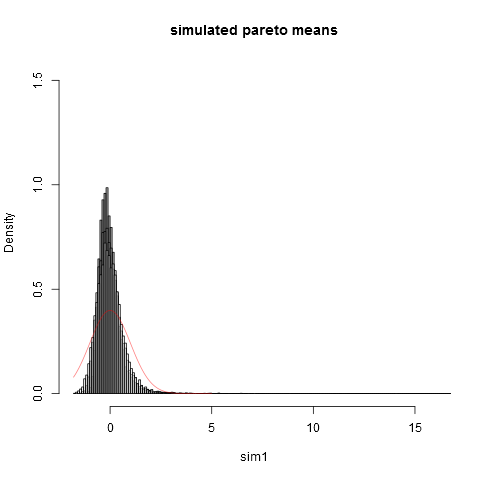
And here is the plot:

One can see that even at sample size $n=10000$ we are far away from the normal approximation. That the empirical variances are so much lower than the true theoretical variance $\sigma^2=1$ is due to the fact that we have a very large contribution to the variance from parts of the distribution in the extreme right tail that do not show up in most samples. This is to be expected always, when the variance "just barely exists". A practical way to think about that is the following. Pareto distributions is often proposed to model distributions of income (or wealth). The expectation of income (or wealth) will have a very large contribution from the very few billionaires. Sampling with practical sample sizes will have a very small probability of including any billionaires in the sample!

Answer 3

I like already given answers but think they are bit too technical for a "lay person explanation" so I will try something more intuitive (starting by an equation ...).

The mean of density $p$ is defined as: $$ \mu = \int x \cdot p(x) dx $$ So grossly speaking, the mean is the "sum over $x$" of the product between the density at $x$ and $x$ itself. When $x$ tends to infinity the density at $p(x)$ must vanish sufficiently so that the product $x \cdot p(x)$ does not go to infinity (and as a result the sum also). When $p(x)$ does not vanish sufficiently, the product goes to infinity, the integral goes to infinity, $\mu$ does not exist and, finally, $p$ has no mean. This is the case of Pareto for certain parameter values.

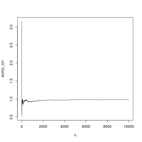
Then, the central limit theorem establishes a distribution of the distance between the empirical mean $\bar{x}=\frac{1}{n} \sum_i x_i$ and the mean $\mu$ as a function of the variance of $p$ and $n$ (asymptotically with $n$). Let see how the empirical mean $\bar{x}$ behaves as a function of the number of $n$ for a Gaussian density $p$:

N=10000;
x=rnorm(N,1,1);
y=rep(NA,N);
for(index in seq(1,N))
{
y[index]=mean(x[1:index])
}
png('~/Desktop/normalMean.png')
plot(y,type='l',xlab='n',ylab='sum(x_i)/n')
dev.off()

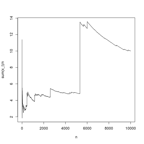
This is a typical realization, the sample mean converges to the density mean quite properly (and in average in the way given by the central limit theorem). Let do the same for a pareto distribution with no mean (substituing rnorm(N,1,1); by pareto(N,1.1,1);)

This is a also a typical simulation, time to time, the sample mean deviates strongly simply because as explained using the integral formula, in the product $p(x) \cdot x$, the frequency of high values of $x$ is no small enough to compensate the fact that $x$ is high. So mean does not exists and the sample mean does not converge to any typical value and the central limit theorem has nothing to say.

Finally, notice that the central limit theorem relates empirical mean, mean, sample size $n$ and variance. So variance $\int (x-\mu)^2 p(x) dx$ must also exists (see kjetil b halvorsen answer for details).