What is the best method of reporting multiple tests of equivalence?

Question

I am doing a study which will involve multiple tests of equivalence. Is there a standard table for reporting such results?

EDIT with more detail: It is a longitudinal study with 5 time points. Our hypothesis is that there is a change from baseline to 1 month and then stability after that. Initially, I thought of a multilevel model but there is no independent variable other than time. So I decided on t-tests between baseline and 1 month and TOST tests of equivalence between 1 and 3 months, 3 and 6, 6 and 9 and 9 and 12.

There were also 5 areas tested.

So, I need a way to summarize all these tests in a table

Answer 1

Regression table presentations are easy enough to modify to accommodate tests for equivalence, including relevance tests—where you base conclusions off of both tests for difference (tests of $H^{^{+}}_{0}$) and tests for equivalence (tests of $H^{^{-}}_{0}$). For example (assuming you are presenting multiple tests in a regression context, hence the $\beta$):

You can present both one-sided test statistics ($t_1$ and $t_2$) and their associated p-values ($p_1$ and $p_2$) from the tests for equivalence, and in addition present the test statistic $t$ and p-value ($p$) for the tests for difference.

In addition you may want to include a column for your definition of equivalence if it varies from test to test (I use $\Delta$ to indicate my equivalence/relevance threshold defined in units of my measures, and $\varepsilon$ to indicate this threshold defined in units of my test statistic). If you use a consistently defined of equivalence/relevance threshold for all tests, you would likely indicate that in a footnote to the table.

You can also facilitate interpretation by including columns to explicitly articulate rejection decisions for equivalence and difference tests. Including a relevance test column (combining results as I have illustrated here) may also facilitate interpretation.

Of course, one can also use this format to present independent tests, and to present different kinds of TOST test statistics (e.g. z test statistics like those used with non-parametric tests, exact binomial test statistics, etc.).

Answer 2

I think one can do all these multiple tests of equivalence within a single linear-mixed models. Given you have multiple (2+) measures after the change took place it is rather natural to present these multiple tests as part of a single repeated-measurements model.

In particular, one could define indicator variables between the successive steps and then check their significance; essentially doing multiple $t$-test in one-go. I think that a random structure with a simple intercept and slope for each subject would be fine. I do not see the absence of independent variables other than time as a structural problem. If anything I think it simplifies matters further.

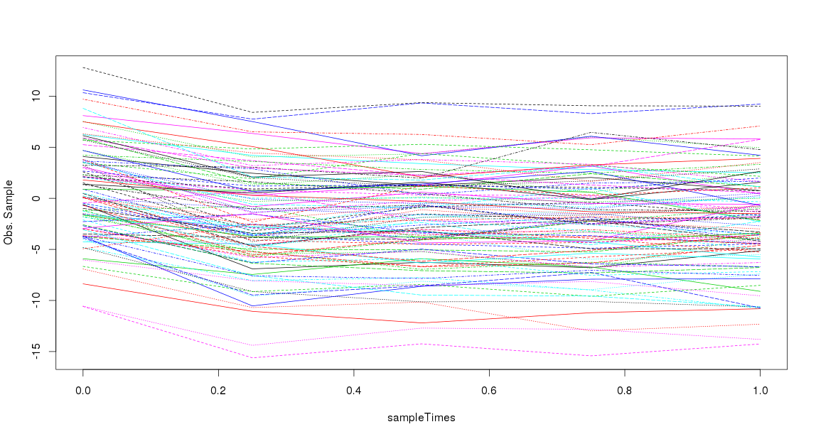
From what I understand given a starting value(val0) something takes place (step0) while stepping from the first measurement period to the second. For the subsequent intra-measurement time periods (step1, step2, step3) nothing happens. Measurement error is assumed constant. So one has something like this:

I create this sample with the following code:

set.seed(123)
sampleTimes <- seq(0,1, length.out = 5); 
N = 10^2;
val0 <- rnorm(N, mean = 0, sd = 5); # Starting values
slopeAt0 <- rnorm( N, mean = -10, sd = 5); # Effect kicks in
val1to5 <- val0 + slopeAt0 * diff(sampleTimes[1:2]) # so val0 is +2.5 higher

trueMeans <- cbind( val0, t(matrix(rep(val1to5,4), 4, byrow = TRUE)))
obsSample <- trueMeans + rnorm(N*5)
subject <- (1:N)
matplot(sampleTimes, t(obsSample),type = 'l', ylab= 'Obs. Sample') # Visualise   

And define a series of indicator variables for the periods stepping from one measurement point to the next. Notice that I define no "last step" step4; we do not know what happens after the last measurement point at $t_4$.

Q <- data.frame( t = rep(sampleTimes, times = N), 
                 ID = rep(subject, each = 5), reads = as.vector(t(obsSample)),
                 step0 = rep(c(1,0,0,0,0), times = N), 
                 step1 = rep(c(0,1,0,0,0), times = N),
                 step2 = rep(c(0,0,1,0,0), times = N), 
                 step3 = rep(c(0,0,0,1,0), times = N))

Using this design it is a relatively simple task to fit an LME and check if the stepX variables become statistically significant. The intercept and slope will absorb any subject-specific variations and one bootstrap that model directly. One can also use the $t$-values from the original LME too.

library(lme4)
m1 <- lmer(reads ~ step0 + step1 + step2 + step3 + (t+1|ID), Q)
summary(m1)
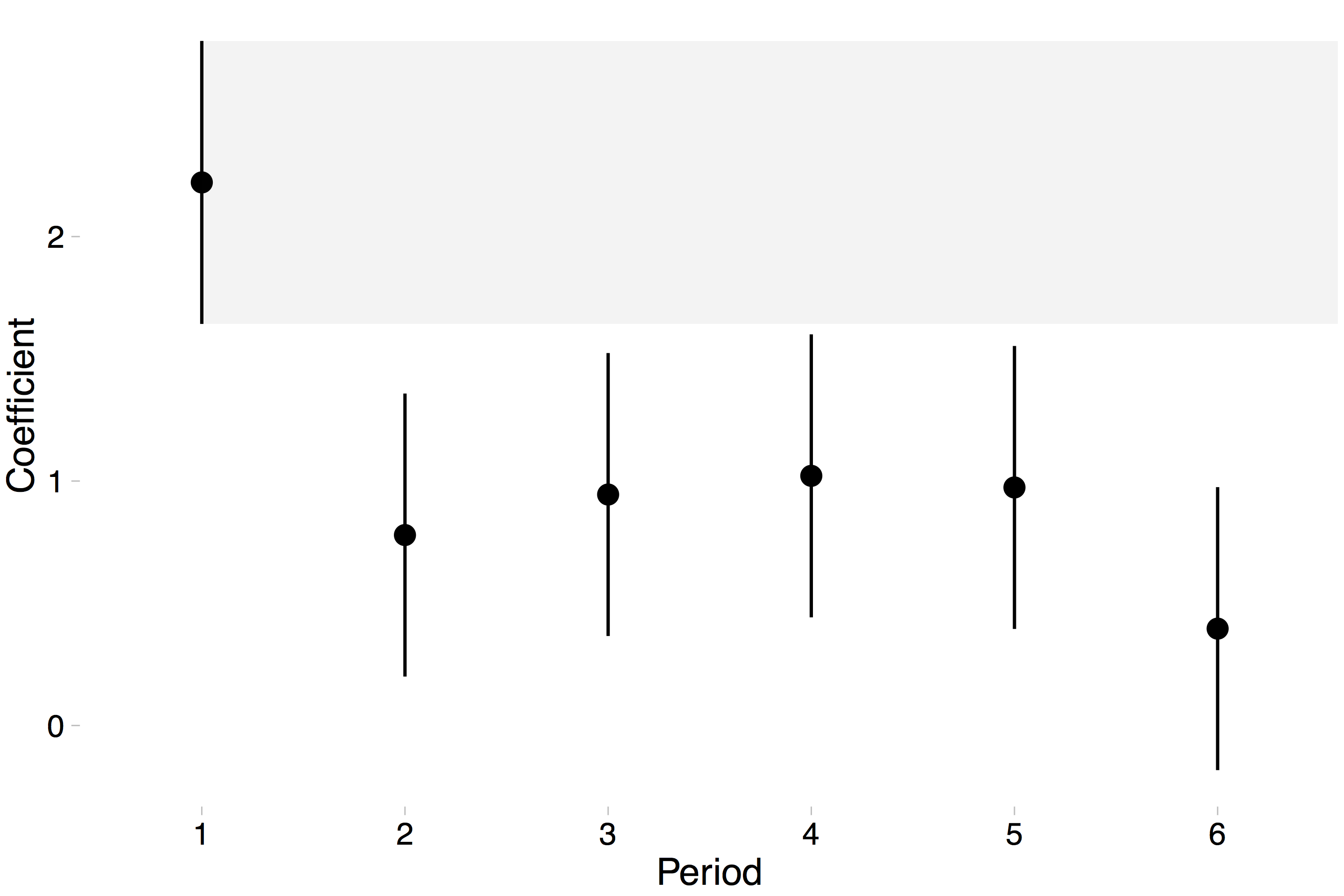
confZ = confint(m1, method='boot', nsim= 1000)
print(confZ)
# Computing bootstrap confidence intervals ...
#                 2.5 %     97.5 %
# .sig01       3.7653500  5.0961341
# .sig02      -0.2043878  0.9843421
# .sig03       0.3396433  1.2702728
# .sigma       0.9869698  1.1579640
# (Intercept) -3.2169570 -1.2982469
# step0        2.5430254  3.2526163
# step1       -0.2465836  0.4475912
# step2       -0.0728649  0.5659132
# step3       -0.1625806  0.4023341

The results are quite reasonable I think, even for the modest sample size ($N = 10^2$) used. Wanting to be on the safe side I included a random slope and this came as probably redundant (sig02) (the original problem description does not specify it there is an additional time-varying trend) but excluding it does not alter the basic findings in any way: something happens during the step0 period.

Answer 3

Others have given you more direct answers to your question, but I'm going to try and show a different solution to the problem. Unless I'm misunderstanding you, it seems like a two-way (period area) fixed effects model would work best (with robust SEs, of course!). $$ y_i = \sum_k \alpha_k \times \mathbf{1}[i \in \text{period}_k] + \sum_j \beta_j \times \mathbf{1}[i \in \text{area}_j] + \epsilon_i $$

You could do an F-test (joint null test) on all the $\alpha_k$ to see if there is any change across time at all, and you can do a Wald test to see if a subset of coefficients (in your case $\alpha_2 = \alpha_3 = \dots = \alpha_K$) are the same. This also gets around all of the multiple testing problems you should be worrying about if you're doing a bunch of pairwise tests.

All of the above can be done within the text. For a visual inspection.. I know you're asking for a table, but I think a plot like this with 95% intervals is much more convincing. But maybe it's just the style of my field.