Can I analyze or model a conditional correlation?

Question

In my research I'm looking at the correlation between self-harm and aggression (both continuous). Now, I also have some variables (e.g. depressive symptoms; also continuous) which I do believe strengthen the relationship between aggression and self-harm. For instance, I believe that self-harm and aggression are more strongly related in people who have more depressive symptoms. How do I test for this?

I though about depressive symptoms being a moderator, but as far as I'm concerned moderators are only appropriate if you look at causal relationships (which I don't, because I look at correlation). Partial correlation also do not seem appropriate cause I want to predict, not control.

As a solution I thought about calculating the correlation coefficients (of aggression and self-harm) for each patient. Then do a multiple regression analysis with depressive symptoms etc. as predictors and the correlation coefficient as outcome variable. But would this be a valid method?

Answer 1

Can I analyze or model a conditional correlation?

This can be done using multivariate regression, which is a form of regression analysis where we have more than one response variable. (Not to be confused with multiple regression, where we have a single response variable but multiple explanatory variables.) A multivariate regression model gives you a predictive equation that predicts all response variables when the explanatory variables in the model are held constant. In this particular case, you could construct a regression model with self-harm and aggression as your two response variables, and depressive_symptoms as the explanatory variable. In R you would use code something like this:

#Construct linear regression for self-harm
#The object DATA is a data frame containing the variables
MODEL <- lm(cbind(self-harm, aggression) ~ depressive_symptoms, data = DATA);

#Extract estimated coefficients and variance matrix of estimates
coef(MODEL);
vcov(MODEL);

Under this model, you will get a fitted model that estimates the coefficients for both of the response variables. Some subsequent mathematics will allow you to determine the estimated correlation between the two response variables when the explanatory variable is held fixed.

Answer 2

You want to study the correlation between self-harm and aggression, but thinks that this might be dependent upon depressive symptoms. One could possibly construct a model for conditional correlation, but I would rather start with some visualization of the data (if you can post a link to data I can include one here).

You have only 170 patients, so the obvious idea of stratification (on depressive symptoms) is difficult to apply. But an extension of that idea to local correlation is possible, effectively using overlapping strata (via weights, as in local regression).

But I would start with visualization: a conditioning plot. There is an R function for that, coplot, and an example of use can be seen here: How do I create and interpret an interaction plot in ggplot2?

(the solution you propose yourself in the last paragraph do not give meaning: You cannot estimate the correlation for each patient (that makes $n=1$), but to estimate a local correlation is an extension/bettering of that idea. It is a variant on the idea of local regression)

I will simulate some data, a bivariate random vector $(X,Y)$ which is bivariate normal, but with a correlation which depends on a third variable $Z$. Such a random vector $(X,Y,Z)$ cannot have a multivariate normal distribution, because then the conditional correlation will be constant. This can be seen using formulas in https://en.wikipedia.org/wiki/Multivariate_normal_distribution#Conditional_distributions.

We need some (inverse) link function mapping an unrestricted variable $z$ to the interval $(-1, 1)$ of possible correlation values. I will use $$ \rho(z) = \frac{e^z-1}{e^z+1}$$(another possibility is Fisher's z transform). Then $Z$ will be standard normal, and $(X,Y) | Z=z$ will be binormal with zero expectation, and covariance matrix $\left(\begin{smallmatrix} 1&\rho(z) \\ \rho(z)&1 \end{smallmatrix}\right)$. Some code for the simulation (R):

library(MASS)

set.seed(7*11*13) # my public seed 
n  <-  1000
z  <-  rnorm(n)  # standard normal
rho  <-  function(z) (exp(z)-1)/(exp(z)+1) #inverse link function for correlation
Sigma <- function(z) matrix( c(1.0, rho(z), rho(z), 1.0), 2, 2)
xy  <-  matrix( rep(0.0, 2*n), n,2 )
for (i in 1:n) {xy[i,]  <-  MASS::mvrnorm(1, mu=rep(0.0,2), Sigma(z[i]))}

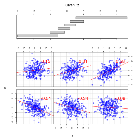
We can show this as a conditioning plot:

The plot should be read starting from the bottom left (order of increasing $z$). Overplotted is a regression line and the Pearson correlation in red. Code for the plot:

mypanel  <-  function(x, y, ...) { r <- cor(x,y) ; points(x,y, ...) ; abline(lm(y ~ x), col="red") ; graphics::text(2.0, 2.0, label=round(r,2), col="red", cex=2.0)  }  
coplot(xy[,2] ~ xy[,1] | z , col="blue", panel=mypanel, xlab="x", ylab="y")

We can show with a hypothesis test that the data is not multinormal:

library(MVN)  # (on CRAN)
xyz <- data.frame(x=xy[,1], y=xy[,2], z=z)
> MVN::mvn(xyz, mvnTest="energy", univariateTest="SW", univariatePlot="qq", multivariatePlot="qq")
$multivariateNormality
         Test Statistic p value MVN
1 E-statistic  2.884006       0  NO

$univariateNormality
          Test  Variable Statistic   p value Normality
1 Shapiro-Wilk     x        0.9987    0.6646    YES   
2 Shapiro-Wilk     y        0.9986    0.6357    YES   
3 Shapiro-Wilk     z        0.9979    0.2621    YES   

(plots not shown).

As a continuation, we could ask if we can formulate a statistical model to estimate a conditional correlation. I have only found explicit references to such ideas in the context of time series, see Dynamic Conditional Correlation (DCC) model yields unexpected sign of fitted correlations. But it is possible to define a model similar to generalized linear models. This is implemented in the R package VGAM (on CRAN), with the family function binormal(). But so far I didn't try it, and will not give examples here. (VGAM can still give the feeling of an experimental, very ambitious project).