Use maximum likelihood.
Generally, suppose you have sorted array of order statistics $x_{[i]}$ for $i$ in a subset $\mathcal{I}$ of $\{1,2,\ldots, n\}$. Augment this vector to include $x_{[0]}=-\infty$ and $x_{[n+1]}=\infty$. You are supposing the underlying distribution is $F_{\theta}$ with corresponding density $f_{\theta}$ and you wish to estimate $\theta$. The likelihood of these order statistics, up to a factor that will not vary with $\theta$, is a product of the $f_\theta{x_{[i]}}$ (excluding $x_{[0]}$ and $x_{[n+1]}$, where necessarily $f=0$) times all the powers
$$\left(F_\theta(x_{[i_{j+1}]}) - F_\theta(x_{[i_j]})\right)^{i_{j+1}-i_j-1}$$
for $j$ from $1$ onward. In the example of the question this would be
$$f_\theta(0)f_\theta(8.1)f_\theta(10)\ \left(F_\theta(8.1) - F_\theta(0)\right)^{949}\left(F_\theta(10) - F_\theta(8.1)\right)^{48}.$$
The rest is completely routine, provided you have at least as many order statistics as there are components of $\theta$: there typically will be a unique value of $\theta$ that minimizes this expression. In the question, $\theta$ has two components and there are three order statistics, so all is fine. The machinery of ML produces, in a standard way, estimated standard errors of the parameters, too.
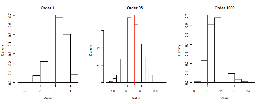
To illustrate, the R code below estimates $\hat\mu=5.39794$ and $\hat\sigma=1.62553$ from the data in the question (namely, $(x_{[1]}, x_{[951]}, x_{[1000]}) = (0, 8.1, 10)$, with $n=1000$). Then, as a quick visual check that the estimates are reasonable, it generates $1000$ datasets of size $n=1000$ from this Normal distribution, records the $1,951,$ and $1000$ order statistics (as given in the question), plots their histograms, and superimposes the observed order statistics on those histograms. The fit is beautiful for orders $1$ and $951$ and reasonable for order $1000$ (the value of $10$ is around the twelfth percentile of this distribution--not too extreme).

#
# Negative log likelihood.
#
Lambda <- function(theta) {
  mu <- theta[1]
  log.sigma <- theta[2]
  sigma <- exp(log.sigma)
  f <- dnorm(values, mu, sigma, log=TRUE)
  F <- log(diff(pnorm(c(-Inf, values, Inf), mu, sigma)))
  -(sum(f) + sum(F * (diff(c(0, orders, n+1))-1)))
}
#
# The data.
#
n <- 1000
orders <- c(1, 951, 1000)
values <- c(0, 8.1, 10)
#
# Compute the estimate.
#
theta.start <- c(mu=mean(range(values)), log.sigma=log(diff(range(values))/6))
fit <- nlm(Lambda, theta.start) # It converged.
theta.hat <- fit$estimate
mu.hat <- theta.hat[1]
sigma.hat <- exp(theta.hat[2])
#
# Check the quality of the estimate visually.
#
n.sim <- 1e3
n <- 1000
sim <- apply(matrix(rnorm(n.sim*n, mu.hat, sigma.hat), n), 2, sort)[orders, ]
par(mfrow=c(1, length(orders)))
invisible(
  sapply(1:length(orders), function(i) {
    hist(sim[i,], freq=FALSE, xlab="Value", main=paste("Order", orders[i]))
    abline(v=values[i], lwd=2, col="Red")
  })
)

