I recently stumbled on the same problem when running arimax function for an intervention analysis on random walk process. i.e. stock price.
The problem we see here is actually by design (of the function itself) as pointed out by Rob Hyndman in his article:
The arimax function from the TSA package fits the transfer function
model (but not the ARIMAX model).
It is not very hard to see from the signature of your function call that you are using TSA::arima, which has exactly the same signature as TSA::arimax and is identical to it (see TSA documentation for details).
This function was by design not to handle ARIMAX model; it was meant for general transfer function-noise model (this is also easy to see from the arguments' naming convention. e.g. xtransf, transfer), which potentially includes some special cases such as 1) regression with ARIMA error, 2) ARMAX model. The only difference between ARMAX and ARIMAX is the integrated part. Here we are basically saying TSA::arima can only take stationary data to start with; if your data requires differencing inside TSA::arima, it won't work.
Programmatically, there's if statement inside TSA::arima to forcefully populate fixed before calling stats::arima and when we have a random walk process which needs differencing (and essentially has nothing to fix), the underlying function stats::arima would correctly complain (discussed below in details).
It is important to note that our model is indeed ARIMAX because we need to difference our data first; if we pass in a differenced version it'll be ARMAX. To be more specific, our data can potentially be modeled by either ARMAX or regression with ARIMA error, because intervention analysis is an application of transfer function model. But it is more the former in our case. ($r=1, s=0$)
Compare:
$$y_{t} = \frac{\beta}{\phi(B)}x_{t} + \frac{\theta(B)}{\phi(B)}z_{t} \qquad\qquad 1.1$$
$$y_{t}=\beta x_{t} + \frac{\theta(B)}{\phi(B)}z_{t} \qquad\qquad\qquad 1.2$$
with:
$$r=1, s=0 \rightarrow y_{t} = \frac{\omega_{0}}{1-\delta B}x_{t} + \frac{\theta(B)}{\phi(B)}N_{t} \qquad\qquad 2.1 $$
$$r=0, s=0 \rightarrow y_{t} = \omega_{0}x_{t} + \frac{\theta(B)}{\phi(B)}N_{t} \qquad\qquad 2.2 $$
It is not hard to see $2.1$ resembles $1.1$ more than $1.2$.
$1.1$ is ARMAX, $1.2$ is regression with ARMA error.
Permutations up to $r=2, s=2$ can be found in Montgomery, Jennings, and Kulahchi (2015).
-------------above concludes the short version of this answer-----------
Therefore, simply adding fixed argument into stats::arima won't cut it as that is not the function we are dealing with here. It helps to learn how it works nonetheless. For reference, stats::arima is the underlying function called from TSA::arima to fit the ARMA error.
P.S. Code example is readily runnable requiring just historic EOD data of AMD, which is easily accessible from Yahoo Finance.
require(TSA)

amd <- read.csv('data/AMD.csv', header = T)
amd.ts <- ts(amd$Close, start=c(2018,5,1), end=c(2019,5,1), frequency = 365)
par(mfrow=c(2,1))
acf(amd.ts);pacf(amd.ts) # check the non-stationarity
m <- stats::arima(amd.ts, order=c(0,1,0)) # ARIMA(0,1,0) for random walk
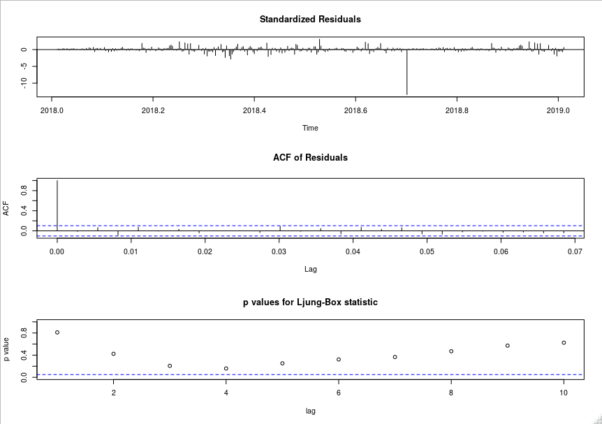
tsdiag(m) # shows ARIMA(0,1,0) is a reasonable fit for our data

For interpretation of the fractional lags, look here
Now comes the interesting part. let's manually fit the data by taking the first difference of log-transformed data (log transform is not required to fit a random walk model to our data) i.e. the log return in financial time series analysis. It is now transformed to ARIMA(0,1,0), by hand.
amd.rw <- diff(log(amd.ts))
m1 <- stats::arima(amd.rw)
# output
# Coefficients:
#       intercept
#          0.0025
# s.e.     0.0033

# sigma^2 estimated as 0.003958:  log likelihood = 491.68,  aic = -979.36
Indeed, stock price tends to show a random walk model with drift (Tsay, 2010):
$$p_{t}=\mu+p_{t-1}+a_{t}, a_{t}\sim N(0, \sigma^2)$$
and $\mu = 0.0025$ in our case.
But why intercept is the only coefficient? that's because we took the first difference of the data, essentially the model looks like:
$$p_{t} - p_{t-1} = \mu + a_{t}$$
there's no parameter left apart from the intercept! Now if we insist fixing some values when in reality there's nothing to fix, it is certainly not sane. This is why I say stats::arima would correctly complain.
Now because R includes intercept as a parameter, we could still fix it by:
m2 <- stats::arima(amd.rw, fixed = c(0.0025))
or any value you like because we are "fixing" it:
m2 <- stats::arima(amd.rw, fixed = c(0))
Bear in mind though, differencing data before passing it to stats::arima makes a difference.
The conclusion here is, if we know the data can be fitted by a simple random walk without drift, passing any value to fixed argument would cause the error.
let's take demeaned data for example:
m3 <- stats::arima(amd.ts - 0.0025, order=c(0,1,0), fixed=c(0))
Error in stats::arima(amd.ts - 0.0025, order = c(0, 1, 0), fixed = c(0)) :
  wrong length for 'fixed'
because TSA::arima force-feeds stats::arima with some fixed values when we have a random walk process, stats::arima doesn't like it as we illustrated above. That being said, they probably didn't intend to consider ARIMAX when they designed the function in the very first place.

