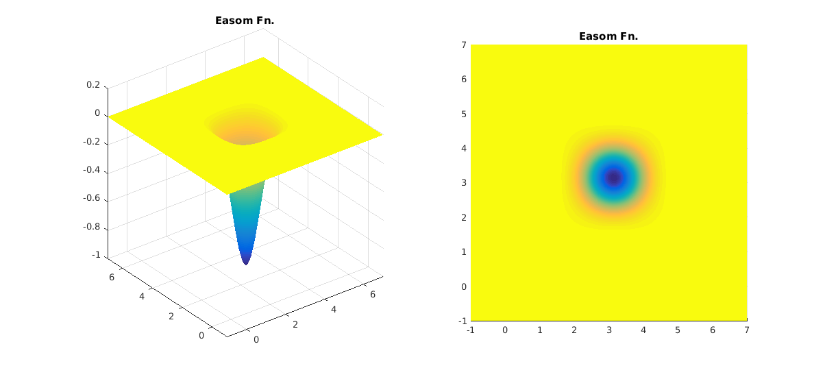
First of all as @whuber mentioned many people are involved in non-convex optimisation. Having said, your definition of "as long as the local minimum is the global minimum" is rather... lax. See for instance the Easom function ($f(x,y) = -\cos(x)\cos(y)\exp(-(x-\pi)^2 - (y-\pi)^2)$. It has a single minimum if that is your concern but if your even remotely away from it you are... staffed. Standard gradient-based methods like BFGS (BFGS in R's optim )and Conjugate Gradient (CG in R's optim) will suffer greatly. You will have to essentially make an "educated guess" about your answer (eg. Simulated Annealing - SANN in R's optim), which a very computationally expensive routine. 
In R:
easom <- function(x){
  -cos(x[1]) * cos(x[2]) * exp( -(x[1] -pi)^2 - (x[2] - pi)^2)
}
optim(easom,par=c(0,0), method='BFGS')$par # 1.664149e-06 1.664149e-06 # Junk
optim(easom,par=c(0,0), method='CG')$par # 0 0 # Insulting Junk
optim(easom,par=c(0,0), method='SANN')$par # 3.382556 2.052309 # Some success!
There are other even worse surfaces to optimise against. See for example Michalewicz's or Schwefel's functions where you might have multiple local minima and/or flat regions.
This flatness is a real problem. For example in generalised as well as standard linear mixed effects model as the number of estimation parameters increases, the log-likelihood function, even after profiling out the residual variance and the fixed-effects parameters can still be very flat. This will lead the model to converge on the boundary of the parameter space or simply to a suboptimal solution (this is actually one of the reason some people myself included are skeptical with the 'keep it maximal' idea for LME's). Therefore "how much convex" your objective function might have big impact to your model as well as your later inference.


