How should I report the results from a mixed model with vs without an interaction term?

Question

In relation to my previous question on different output results and their interpretation based on a model with or without an interaction term, this is a follow up question on how to report such results.

Based on the following model formula and its output (see below), am I correct at interpreting this no-interaction model as follows;

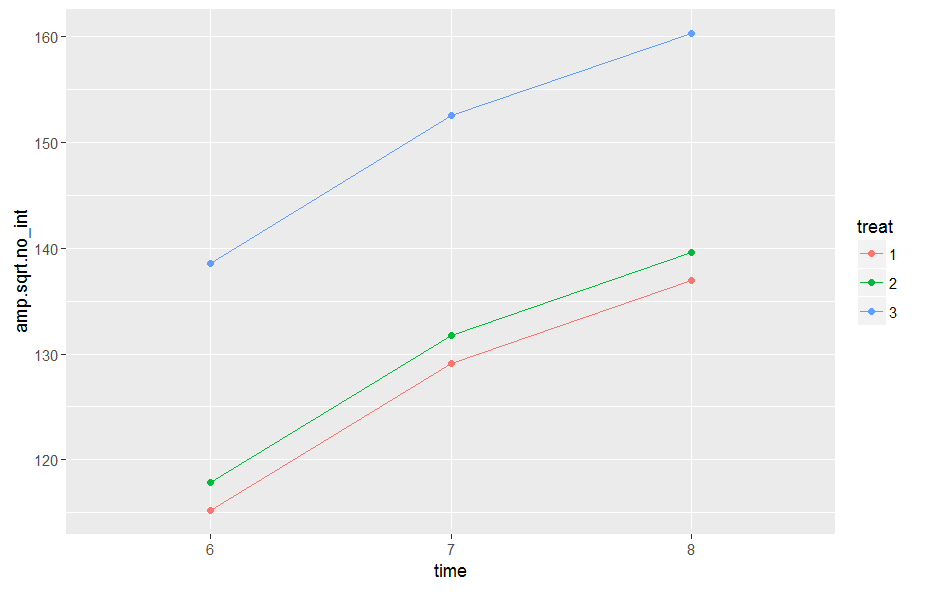
For treatment1 at time6, we have amp.sqrt = 115.184

For treatment2 at time6, we have amp.sqrt = 115.184 + 2.644

For treatment3 at time6, we have amp.sqrt = 115.184 + 23.365

For treatment1 at time7, we have amp.sqrt = 115.184 + 13.958

For treatment2 at time7, we have amp.sqrt = 115.184 + 13.958 + 2.644

For treatment3 at time7, we have amp.sqrt = 115.184 + 13.958 + 23.365

etc..

I had thought of reporting the results as: "there was a positive effect of treatment, with amp.sqrt increasing from treatment 1, to 2 (2.644) and 3 (23.365). Also a positive effect of time was observed, increasing from time 1 to 2 (13.958) and 3 (21.799). The main effect of axis increased from 1 to 2 and 3 as well."

However, now that I have my model with the interaction term, and the main effects on their own seem strange to report (as I wrote above), should I instead report the overall trends as seen by your plot (i.e. adding the fixed effects and the interaction term and then presenting that value) or should I still present the results as above, even if the main effect outputs on their own are counterintuitive unless specified in relation with the interaction term results?

(NO-INTERACTION TERM MODEL)
mTEST1<- lmer(amp.sqrt~ time + treatment + axis + (1+treatment|ID))

Fixed effects:
        Estimate Std. Error      df t value Pr(>|t|)    
(Intercept)  115.184      7.546  36.300  15.265  < 2e-16 ***
time7         13.958      4.707 474.800   2.965  0.00318 ** 
time8         21.799      4.787 478.500   4.554  6.7e-06 ***
treatment2     2.644      8.571  18.400   0.308  0.76117    
treatment3    23.365      6.139  19.200   3.806  0.00117 ** 
axis2         60.458      4.746 474.800  12.737  < 2e-16 ***
axis3        128.456      4.746 474.800  27.063  < 2e-16 ***
---

(INTERACTION-TERM MODEL)
mTEST2<- lmer(amp.sqrt~ time * treatment + axis + (1+treatment|ID))

Fixed effects:
                 Estimate Std. Error      df t value Pr(>|t|)    
(Intercept)       130.587      8.417  55.500  15.515  < 2e-16 ***
time7              -7.697      8.120 471.000  -0.948   0.3436    
time8              -2.628      8.120 471.000  -0.324   0.7464    
treatment2         -3.766     10.713  44.500  -0.352   0.7269    
treatment3        -14.929      8.851  83.600  -1.687   0.0954 .  
axis2              60.458      4.569 471.000  13.232  < 2e-16 ***
axis3             128.456      4.569 471.000  28.113  < 2e-16 ***
time7:treatment2    9.697     11.206 471.000   0.865   0.3873    
time8:treatment2    8.554     11.396 473.700   0.751   0.4532    
time7:treatment3   53.206     11.206 471.000   4.748 2.73e-06 ***
time8:treatment3   62.411     11.289 473.300   5.528 5.35e-08 ***

Answer 1

First of all, yes, you are correct in the way you are interpreting the fixed effects.

However, note that we are only dealing here with fixed effects. Your model also has random effects, and in particular you have random coefficients for treatment which means that each subject has their own individual treatment effect. The calculations with the fixed effects therefore represent averages across all subjects.

Although the findings are largely the same, I would present your findings based on the model with the interactions. We can view the model with no interactions with this plot:

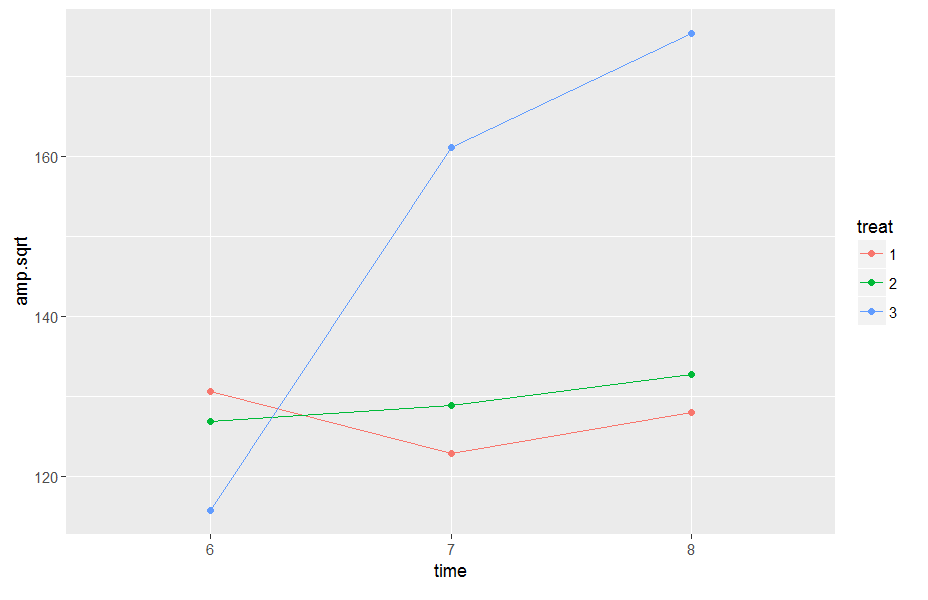
While the model with interactions looks like this:

Formally, you can do a likelihood ratio test using the anova() function to test which model is better (you will have to re-run your models using the REML=FALSE option because likelihood-based methods cannot be used to compare models with different fixed effects).

I would focus on treatment 3 being associated with higher values of amp.sqrt at time 7 and further at time 8, and these differences are also statistically significant at the 5% level. Treatment 3 is associated with lower values at time 6 (although this difference is not statistically significant at the 5% level). Also, there is very little differences between treatments 1 and 2 at all time points (and these are also not statistically significant). Moreover there appears to be no time trend for treatments 1 and 2. You might be interested in a test of whether treatment 2 is different between years 6 and 8 since there is a small upward trend. Personally this looks negligible to me, compared with treatment 3 but if you wanted to test this you could use a post-hoc test such as Dunnett's.