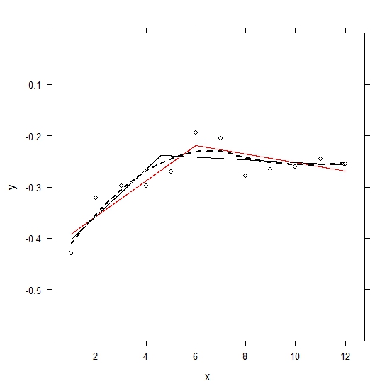
I estimated the breakpoint for a piecewise linear model (one intercept, two slopes that meet at the breakpoint) by minimizing the deviance using an optimizer (optim in R). I noticed that the estimate was near 2.0, 4.0, and 6.0, depending on the initial conditions, indicating there were local optima. So I used simulated annealing to estimate the breakpoint (optim(..., method="SANN", ...)), and became reasonably confidence that I had found the globally best estimate at bp = 6.0. I just finished bootstrapping the breakpoint estimates (my data are nested within subjects, and I had to apply simulated annealing to each bootstrap estimate, so the whole thing took a couple days), and found that:
1) The bootstrap distribution is bimodal, with modes at 2.0 and 6.0.
2) The mean of the bootstrap distribution is 4.0, and the median is 3.5, whereas the parameter estimate was 6.0.
Can someone help me to understand my results? I want to say that the original estimate of 6.0 is an artifact of my sample, and that the bootstrap mean of 4.0 is a better estimate of the breakpoint, but I'm not sure if this is the right interpretation. Also, placing the breakpoint at 4.0 produces conditional means that agree almost exactly with a LOESS curve using default values (a breakpoint at 6.0 does not agree as well).
--
Edit: Adding a graph.

Figure notes: Red line = original fit with bp = 6.0. Black solid = fit with bp = 4.6. Black dotted = LOESS. Open circles = means. Models were fit to full data set (too many data points to show, and yes, I tried high density plotting methods as well), not means.
