2
$\begingroup$

Suppose that I am working with an integer-valued variable $x$ and that all I know about my sample is as follows:

  • Mean $\bar{x}$: 4.5
  • Sample size $n$: 100
  • I can safely assume that the underlying model for this data is Poisson. However, it is a truncated distribution as the variable can only take on values 1, 2, 3, 4 and 5 (think of the product ratings given by customers in their online reviews).

The end goal is to estimate the $\lambda$ parameter of that Poisson distribution and use it to simulate a predictive distribution for $x$.

If it wasn't a truncated Poisson distribution, I could assume that the prior of $\lambda$ is a Gamma distribution, $\Gamma(\alpha, \beta)$. Then the posterior distribution would be $\Gamma(\alpha + n \bar{x}, \beta + n)$. With a non-informative Gamma distribution, i.e. $\Gamma(0, 0)$, that would lead to $\lambda = \Gamma(450, 100)$ (see pp. 65-66 in this work for reasoning on the non-informative prior Gamma). Using this posterior, I could then easily simulate the predictive distribution in R as follows:

lambda <- rgamma(10000, 450, 100)
x <- rpois(10000, lambda)

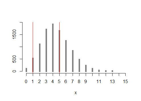
However, plotting this simulated values immediately reveals that many of them are outside of the 1-5 interval:

plot(table(x), 
     type = "h", lwd = 5,
     lend = 2, 
     col = gray(0.5), 
     bty = "n",
     ylab = "")

enter image description here

Again, this plot doesn't come as a big surprise as the math used to produce it assumed a non-truncated Poisson distribution for $x$. Now the question is: how can I modify that math so that the resulting predictive distribution is bounded by 1 on the lower end and by 5 on the upper end? An answer with an example R code would be greatly appreciated.

$\endgroup$
2
  • 1
    $\begingroup$ Having the data truncated does not imply the parameter is to be truncated. $\endgroup$
    – Xi'an
    Commented Sep 8, 2016 at 16:40
  • $\begingroup$ Why not estimate the parameter with the EM algorithm? $\endgroup$
    – AdamO
    Commented Sep 8, 2016 at 16:52

1 Answer 1

6
$\begingroup$

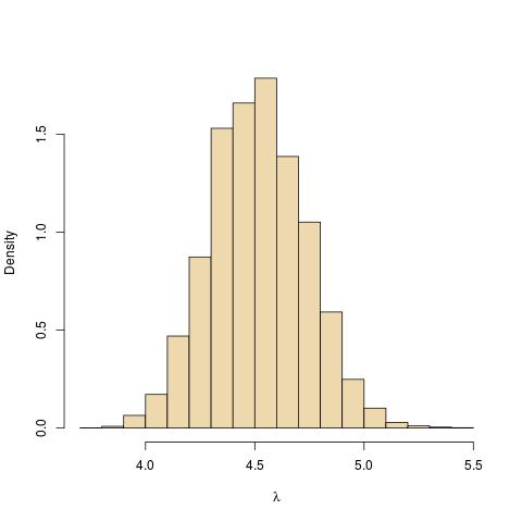
If the $x_i$'s are truncated Poisson $P(\lambda)$, then their pdf is $$p(x)=\dfrac{\lambda^x\exp\{-\lambda\}}{x!\mathbb{P}_\lambda(1\le X\le 5)}$$Hence, the posterior distribution associated with the Jeffreys prior $\pi(\lambda)=1/\lambda$ is $$\pi(\lambda|\bar{x}_n)\propto \dfrac{\lambda^{n\bar{x}_n}\exp\{-n\lambda\}}{\lambda\mathbb{P}_\lambda(1\le X\le 5)^n}$$While non-standard it remains manageable by a Metropolis-Hastings or even an accept-reject algorithm.

MCMC representation of the posterior distribution on <span class=$\lambda$">

For instance, here is my R code

n=100
barx=n*4.5-1

like=function(lam){ barx*log(lam)-n*lam-n*log(ppois(5,lam)-ppois(0,lam))}

T=1e4
mcmc=rep(barx/n,T)
a=barx*.1
b=n*.1

for (t in 2:T){

mcmc[t]=prop=rgamma(1,a,rate=b)
if (log(runif(1))>like(prop)-like(mcmc[t-1])-dgamma(prop,a,rate=b,log=TRUE)+
    dgamma(mcmc[t-1],a,rate=b,log=TRUE)) mcmc[t]=mcmc[t-1]}
$\endgroup$
1
  • $\begingroup$ thank you very much. If only someone could help me translate that into code now. I'm afraid my knowledge of Bayesian stats stops at simple situations like the one I described in the original question. Off to do more reading... $\endgroup$
    – Syarzhuk
    Commented Sep 8, 2016 at 18:52

Your Answer

By clicking “Post Your Answer”, you agree to our terms of service and acknowledge you have read our privacy policy.

Not the answer you're looking for? Browse other questions tagged or ask your own question.