Bayesian updating with new data

Question

How do we go about calculating a posterior with a prior N~(a, b) after observing n data points? I assume that we have to calculate the sample mean and variance of the data points and do some sort of calculation that combines the posterior with the prior, but I'm not quite sure what the combination formula looks like.

Answer 1

The basic idea of Bayesian updating is that given some data $X$ and prior over parameter of interest $\theta$, where the relation between data and parameter is described using likelihood function, you use Bayes theorem to obtain posterior

$$ p(\theta \mid X) \propto p(X \mid \theta) \, p(\theta) $$

This can be done sequentially, where after seeing first data point $x_1$ prior $\theta$ becomes updated to posterior $\theta'$, next you can take second data point $x_2$ and use posterior obtained before $\theta'$ as your prior, to update it once again etc.

Let me give you an example. Imagine that you want to estimate mean $\mu$ of normal distribution and $\sigma^2$ is known to you. In such case we can use normal-normal model. We assume normal prior for $\mu$ with hyperparameters $\mu_0,\sigma_0^2:$

\begin{align} X\mid\mu &\sim \mathrm{Normal}(\mu,\ \sigma^2) \\ \mu &\sim \mathrm{Normal}(\mu_0,\ \sigma_0^2) \end{align}

Since normal distribution is a conjugate prior for $\mu$ of normal distribution, we have closed-form solution to update the prior

\begin{align} E(\mu' \mid x) &= \frac{\sigma^2\mu + \sigma^2_0 x}{\sigma^2 + \sigma^2_0} \\[7pt] \mathrm{Var}(\mu' \mid x) &= \frac{\sigma^2 \sigma^2_0}{\sigma^2 + \sigma^2_0} \end{align}

Unfortunately, such simple closed-form solutions are not available for more sophisticated problems and you have to rely on optimization algorithms (for point estimates using maximum a posteriori approach), or MCMC simulation.

Below you can see data example:

n <- 1000
set.seed(123)
x     <- rnorm(n, 1.4, 2.7)
mu    <- numeric(n)
sigma <- numeric(n)

mu[1]    <- (10000*x[i] + (2.7^2)*0)/(10000+2.7^2)
sigma[1] <- (10000*2.7^2)/(10000+2.7^2)
for (i in 2:n) {
  mu[i]    <- ( sigma[i-1]*x[i] + (2.7^2)*mu[i-1] )/(sigma[i-1]+2.7^2)
  sigma[i] <- ( sigma[i-1]*2.7^2                  )/(sigma[i-1]+2.7^2)
}

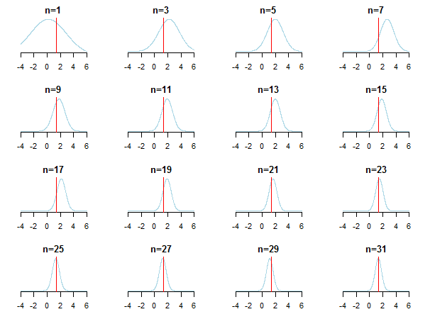
If you plot the results, you'll see how posterior approaches the estimated value (it's true value is marked by red line) as new data is accumulated.

For learning more you can check those slides and Conjugate Bayesian analysis of the Gaussian distribution paper by Kevin P. Murphy. Check also Do Bayesian priors become irrelevant with large sample size? You can also check those notes and this blog entry for accessible step-by-step introduction to Bayesian inference.

Answer 2

If you have a prior $P(\theta)$ and a likelihood function $P(x \mid \theta)$ you can calculate the posterior with:

$$ P(\theta \mid x) = \frac{\sum_\theta P(x \mid \theta) P(\theta)}{P(x)} $$

Since $P(x)$ is just a normalization constant to make probabilities sum to one, you could write:

$$P(\theta \mid x) \sim \sum_\theta P(x \mid \theta)P(\theta) $$

Where $\sim$ means "is proportional to."

The case of conjugate priors (where you often get nice closed form formulas)

This Wikipedia article on conjugate priors may be informative. Let $\boldsymbol{\theta}$ be a vector of your parameters. Let $P(\boldsymbol{\theta})$ be a prior over your parameters. Let $P(\mathbf{x} \mid \boldsymbol{\theta})$ be the likelihood function, the probability of the data given the parameters. The prior is a conjugate prior for the likelihood function if the prior $P(\boldsymbol{\theta})$ and the posterior $P(\boldsymbol{\theta} \mid \mathbf{x})$ are in the same family (eg. both Gaussian).

The table of conjugate distributions may help build some intuition (and also give some instructive examples to work through yourself).

Answer 3

This is the central computation issue for Bayesian data analysis. It really depends on the data and distributions involved. For simple cases where everything can be expressed in closed form (e.g., with conjugate priors), you can use Bayes's theorem directly. The most popular family of techniques for more complex cases is Markov chain Monte Carlo. For details, see any introductory textbook on Bayesian data analysis.