Does clustering lead to overdispersion?

Question

TL;DR

Clustering is often cited as a source of overdispersion in count data. However, I seem to arrive at the conclusion that clustering actually reduces the dispersion.

Could someone confirm this or show me where I am wrong?

Model

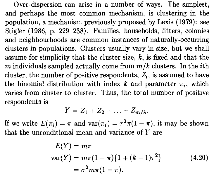
Here's an excerpt from "Generalized Linear Models" by McCullagh and Nelder:

It is my understanding that $\pi_i$ here is considered a set of fixed parameters along with $k$ and $m$ (i.e. this is not a hierarchical model), where $E(\pi_i)$ and $\mathrm{var}(\pi_i)$ refer to the sample mean and variance of the set of fixed numbers $\{\pi_1,\ldots,\pi_{m/k}\}$.

My results

Under the above assumptions, the variance I arrive at is

$$\mathrm{var}(Y)=m(\pi(1-\pi)-\mathrm{var}(\pi_i)),$$

which is smaller than the variance of $\mathrm{Binom}(m,\pi)$.

This also makes intuitive sense, since variance of the binomial distribution is a concave function of the mean, and so spreading out the $\pi_i$'s reduces the variance.

Finally, I made a quick simulation in R that further confirms it:

> set.seed(2016+10+21)
> m <- 100
> k <- 5
> p <- runif(m/k)
> p_m <- mean(p)
> p_v <- mean((p-p_m)^2)
> # Simulated variance
> mean(replicate(1000, var(replicate(50, sum(rbinom(m/k, k, p))))))
[1] 17.69588
> # My formula for clustered variance
> m*(p_m*(1-p_m)-p_v)
[1] 17.59746
> # Non-clustered variance
> m*(p_m*(1-p_m))
[1] 24.84612

So, could someone confirm this or show me where I am wrong?

Answer 1

First, regarding this comment by the OP

It is my understanding that $\pi_i$ here is considered a set of fixed parameters along with $k$ and $m$ (i.e. this is not a hierarchical model), where $\mathbb E (\pi_i)$ and $\text{var}(\pi_i)$ refer to the sample mean and variance of the set of fixed numbers $\{\pi_1,\dots,\pi_{m/k}\}$.

Mathematically, there is no difference between the two, the latter is also a hierarchical model, albeit with a special distribution for $\pi_i$, namely the empirical distribution of a finite sample.

The model is $Z_i \mid \pi_i \sim \text{Bin}(k, \pi_i)$, hence $\mathbb E(Z_i \mid \pi_i) = k \pi_i$ and $\text{var}(Z_i \mid \pi_i) = k \pi_i(1-\pi_i)$. Then, the law of total variance gives \begin{align*} \text{var}(Z_i) &= \mathbb E[ \text{var}(Z_i \mid \pi_i)] + \text{var}(\mathbb E[Z_i \mid \pi_i]) \\ &= \mathbb E[k \pi_i(1-\pi_i)] + \text{var}(k \pi_i) \\ &=k \big[\mathbb E[\pi_i] - \mathbb E [\pi_i^2] \big] + k^2 \text{var}(\pi_i)\\ &= k\big[ \pi - (\pi^2 + \tau^2\pi(1-\pi))\big] + k^2 \tau^2 \pi(1-\pi) \\ &= k\big[ \pi(1-\pi) - \tau^2\pi(1-\pi))\big] + k^2 \tau^2 \pi(1-\pi) \\ &= k \pi(1-\pi)[1 - \tau^2 +k \tau^2] \\ &= k\pi(1-\pi)[1 + (k-1)\tau^2]. \end{align*} Since $\text{var}(Z_i)$ is the same for all $i$, and $Z_i$ are independent, we have \begin{align*} \text{var}(Y) = \text{var}\Big( \sum_{i=1}^{m/k} Z_i\Big) = \sum_{i=1}^{m/k} \text{var}(Z_i) &= \frac{m}{k}k\pi(1-\pi)[1 + (k-1)\tau^2] \\ &= m\pi(1-\pi)[1 + (k-1)\tau^2]. \end{align*} So, McCullagh and Nelder are right about it.