9
$\begingroup$

I was reading this page on Princeton.edu. They are performing a logistic regression (with R). At some point they calculate the probability of getting a residual deviance higher than the one they got on a $\chi^2$ distribution with degrees of freedom equal to the degrees of freedom of the model. Copying-pasting from their website...

> glm( cbind(using,notUsing) ~ age + hiEduc + noMore, family=binomial)

Call:  glm(formula = cbind(using, notUsing) ~ age + hiEduc + noMore,      
     family = binomial) 

Coefficients:
(Intercept)     age25-29     age30-39     age40-49       hiEduc       noMore  
    -1.9662       0.3894       0.9086       1.1892       0.3250       0.8330  

Degrees of Freedom: 15 Total (i.e. Null);  10 Residual
Null Deviance:      165.8 
Residual Deviance: 29.92        AIC: 113.4 

The residual deviance of 29.92 on 10 d.f. is highly significant:

> 1-pchisq(29.92,10)
[1] 0.0008828339

so we need a better model


Why does it make sense to compute 1-pchisq(29.92,10) and why does a low probability indicate that something is going wrong with their model?

$\endgroup$

3 Answers 3

8
$\begingroup$

They are using a deviance test shown below: $$ D(y) = -2\ell(\hat\beta;y) + 2\ell(\hat\theta^{(s)};y) $$

Here the $\hat β$ represents the fitted model of interest and $\hatθ(s)$ represents the saturated model. The log-likelihood for the saturated model is (more often than not) $0$, hence you are left with the residual deviance of the model they fitted ($29.92$). This deviance test is approximately chi-squared with degrees of freedom $n-p$ ($n$ being the observations and $p$ being the number of variables fitted). You have $n=16$ and $p=6$ so the test will be approximately $\chi^2_{10}$. The null of the test is that your fitted model fits the data well and there is no misfit—you haven't missed any sources of variation. In the above test you reject the null and, as a result, you have missed something in the model you fitted. The reason for using this test is that the saturated model will fit the data perfectly so if you were in the case where you are not rejecting the null between your fitted model and the saturated model, it indicates you haven't missed big sources of data variation in your model.

$\endgroup$
3
$\begingroup$

Your question, as stated, has been answered by @francium87d. Comparing the residual deviance against the appropriate chi-squared distribution constitutes testing the fitted model against the saturated model and shows, in this case, a significant lack of fit.


Still, it might help to look more thoroughly at the data and the model to understand better what it means that the model has a lack of fit:

d = read.table(text=" age education wantsMore notUsing using 
   <25       low       yes       53     6
   <25       low        no       10     4
   <25      high       yes      212    52
   <25      high        no       50    10
 25-29       low       yes       60    14
 25-29       low        no       19    10
 25-29      high       yes      155    54
 25-29      high        no       65    27
 30-39       low       yes      112    33
 30-39       low        no       77    80
 30-39      high       yes      118    46
 30-39      high        no       68    78
 40-49       low       yes       35     6
 40-49       low        no       46    48
 40-49      high       yes        8     8
 40-49      high        no       12    31", header=TRUE, stringsAsFactors=FALSE)
d = d[order(d[,3],d[,2]), c(3,2,1,5,4)]

library(binom)
d$proportion = with(d, using/(using+notUsing))
d$sum        = with(d, using+notUsing)
bCI          = binom.confint(x=d$using, n=d$sum, methods="exact")

m     = glm(cbind(using,notUsing)~age+education+wantsMore, d, family=binomial)
preds = predict(m, new.data=d[,1:3], type="response")

windows()
  par(mar=c(5, 8, 4, 2))
  bp = barplot(d$proportion, horiz=T, xlim=c(0,1), xlab="proportion",
               main="Birth control usage")
  box()
  axis(side=2, at=bp, labels=paste(d[,1], d[,2], d[,3]), las=1)
  arrows(y0=bp, x0=bCI[,5], x1=bCI[,6], code=3, angle=90, length=.05)
  points(x=preds, y=bp, pch=15, col="red")
enter image description here

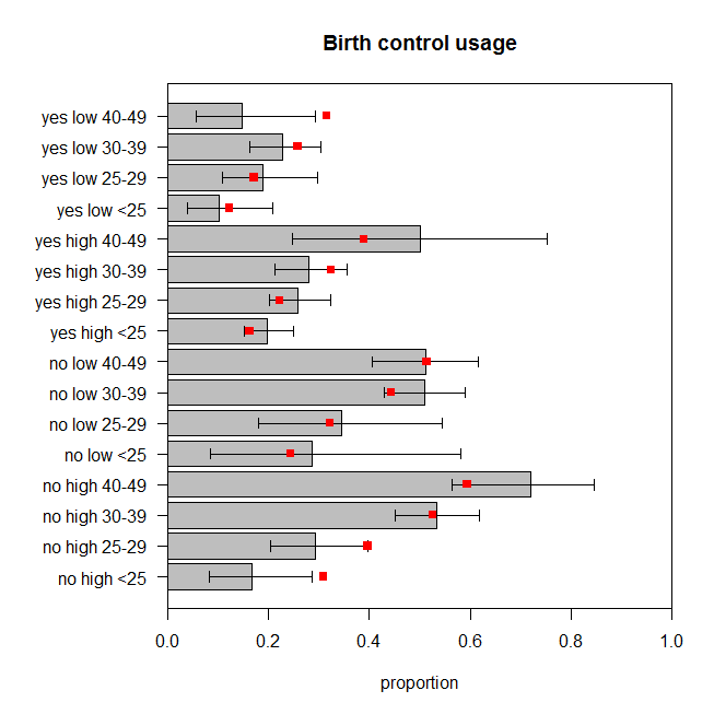
The figure plots the observed proportion of women in each set of categories that are using birth control, along with the exact 95% confidence interval. The model's predicted proportions are overlaid in red. We can see that two predicted proportions are outside of the 95% CIs, and anther five are at or very near the limits of the respective CIs. That's seven out of sixteen ($44\%$) that are off target. So the model's predictions don't match the observed data very well.

How could the model fit better? Perhaps there are interactions amongst the variables that are relevant. Let's add all the two-way interactions and assess the fit:

m2 = glm(cbind(using,notUsing)~(age+education+wantsMore)^2, d, family=binomial)
summary(m2)
# ...
#     Null deviance: 165.7724  on 15  degrees of freedom
# Residual deviance:   2.4415  on  3  degrees of freedom
# AIC: 99.949
# 
# Number of Fisher Scoring iterations: 4
1-pchisq(2.4415, df=3)  # [1] 0.4859562
drop1(m2, test="LRT")
# Single term deletions
# 
# Model:
# cbind(using, notUsing) ~ (age + education + wantsMore)^2
#                     Df Deviance     AIC     LRT Pr(>Chi)  
# <none>                   2.4415  99.949                   
# age:education        3  10.8240 102.332  8.3826  0.03873 *
# age:wantsMore        3  13.7639 105.272 11.3224  0.01010 *
# education:wantsMore  1   5.7983 101.306  3.3568  0.06693 .

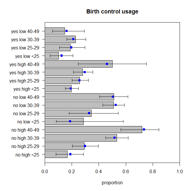
The p-value for the lack of fit test for this model is now $0.486$. But do we really need all those extra interaction terms? The drop1() command shows the results of the nested model tests without them. The interaction between education and wantsMore is not quite significant, but I would be fine with it in the model anyway. So let's see how the predictions from this model compare to the data:
enter image description here

These aren't perfect, but we shouldn't assume that the observed proportions are a perfect reflection of the true data generating process. These look to me like they are bouncing around the appropriate amount (more correctly that the data are bouncing around the predictions, I suppose).

$\endgroup$
2
$\begingroup$

I do not believe that the residual deviance statistic has a $\chi^2$ distribution. I think it is a degenerate distribution because asymptotic theory does not apply when the degrees of freedom increases at the same speed as the sample size. At any rate I doubt that the test has sufficient power, and encourage directed tests such as tests of linearity using regression splines and tests of interaction.

$\endgroup$
5
  • 1
    $\begingroup$ I think because in this case all the predictors are categorical, the no. degrees of freedom of the saturated model wouldn't increase with sample size, so the asymptotic approach makes sense. The sample size is still rather small though. $\endgroup$
    – Scortchi
    Commented Dec 1, 2016 at 15:19
  • $\begingroup$ Not sure that's it. The d.f. of the model parameters is fixed but the d.f. of the residual "$\chi^2$" is $n$ minus that. $\endgroup$ Commented Dec 1, 2016 at 16:54
  • $\begingroup$ In this case the data consist of 1607 individuals in a contingency table & the test is comparing a 6-parameter model with the 16-parameter saturated model (rather than a 1607-parameter model). $\endgroup$
    – Scortchi
    Commented Dec 1, 2016 at 17:14
  • $\begingroup$ Then it should not be labeled as residual $\chi^2$. $\endgroup$ Commented Dec 1, 2016 at 19:26
  • 1
    $\begingroup$ I agree this terminology's unfortunate: glm gives a different "residual deviance" when the data are grouped up from when they aren't - & a different "null deviance" for that matter. $\endgroup$
    – Scortchi
    Commented Dec 2, 2016 at 10:44

Your Answer

By clicking “Post Your Answer”, you agree to our terms of service and acknowledge you have read our privacy policy.

Not the answer you're looking for? Browse other questions tagged or ask your own question.