Cumming (2008) claims that distribution of p-values obtained in replications depends only on the original p-value. How can it be true?

Question

I have been reading Geoff Cumming's 2008 paper Replication and $p$ Intervals: $p$ values predict the future only vaguely, but confidence intervals do much better [~200 citations in Google Scholar] -- and am confused by one of its central claims. This is one in the series of papers where Cumming argues against $p$-values and in favour of confidence intervals; my question, however, is not about this debate and only concerns one specific claim about $p$-values.

Let me quote from the abstract:

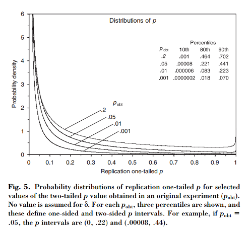
This article shows that, if an initial experiment results in two-tailed $p= .05$, there is an $80\%$ chance the one-tailed $p$-value from a replication will fall in the interval $(.00008, .44)$, a $10\%$ chance that $p < .00008$, and fully a $10\%$ chance that $p > .44$. Remarkably, the interval—termed a $p$ interval—is this wide however large the sample size.

Cumming claims that this "$p$ interval", and in fact the whole distribution of $p$-values that one would obtain when replicating the original experiment (with the same fixed sample size), depend only on the original $p$-value $p_\mathrm{obt}$ and do not depend on the true effect size, power, sample size, or anything else:

[...] the probability distribution of $p$ can be derived without knowing or assuming a value for $\delta$ (or power). [...] We do not assume any prior knowledge about $\delta$, and we use only the information $M_\mathrm{diff}$ [observed between-group difference] gives about $\delta$ as the basis for the calculation for a given $p_\mathrm{obt}$ of the distribution of $p$ and of $p$ intervals.

$\quad\quad\quad$

I am confused by this because to me it seems that the distribution of $p$-values strongly depends on power, whereas the original $p_\mathrm{obt}$ on its own does not give any information about it. It might be that the true effect size is $\delta=0$ and then the distribution is uniform; or maybe the true effect size is huge and then we should expect mostly very small $p$-values. Of course one can start with assuming some prior over possible effect sizes and integrate over it, but Cumming seems to claim that this is not what he is doing.

Question: What exactly is going on here?

---

Note that this topic is related to this question: What fraction of repeat experiments will have an effect size within the 95% confidence interval of the first experiment? with an excellent answer by @whuber. Cumming has a paper on this topic to: Cumming & Maillardet, 2006, Confidence Intervals and Replication: Where Will the Next Mean Fall? -- but that one is clear and unproblematic.

I also note that Cumming's claim is repeated several times in the 2015 Nature Methods paper The fickle $P$ value generates irreproducible results that some of you might have come across (it already has ~100 citations in Google Scholar):

[...] there will be substantial variation in the $P$ value of repeated experiments. In reality, experiments are rarely repeated; we do not know how different the next $P$ might be. But it is likely that it could be very different. For example, regardless of the statistical power of an experiment, if a single replicate returns a $P$ value of $0.05$, there is an $80\%$ chance that a repeat experiment would return a $P$ value between $0$ and $0.44$ (and a $20\%$ change [sic] that $P$ would be even larger).

(Note, by the way, how, irrespective of whether Cumming's statement is correct or not, Nature Methods paper quotes it inaccurately: according to Cumming, it's only $10\%$ probability above $0.44$. And yes, the paper does say "20% change". Pfff.)

Answer 1

Summary: The trick appears to be a Bayesian approach which assumes a uniform (Jeffreys) prior for the hidden parameter ($z_\mu$ in appendix B of the paper, $\theta$ here).

I believe there may be a Bayesian-style approach to get the equations given in the paper's appendix B.

As I understand it, the experiment boils down to a statistic $z\sim\mathrm{N}_{\theta,1}$. The mean $\theta$ of the sampling distribution is unknown, but vanishes under the null hypothesis, $\theta\mid{}H_0=0$.

Call the experimentally observed statistic $\hat{z}\mid\theta\sim\mathrm{N}_{\theta,1}$. Then if we assume a "uniform" (improper) prior on $\theta\sim1$, the Bayesian posterior is $\theta\mid\hat{z}\sim\mathrm{N}_{\hat{z},1}$. If we then update the original sampling distribution by marginalizing over $\theta\mid\hat{z}$, the posterior becomes $z\mid\hat{z}\sim\mathrm{N}_{\hat{z},2}$. (The doubled variance is due to convolution of Gaussians.)

Mathematically at least, this seems to work. And it explains how the $\frac{1}{\sqrt{2}}$ factor "magically" appears going from equation B2 to equation B3.

---

Discussion

How can this result be reconciled with the standard null hypothesis testing framework? One possible interpretation is as follows.

In the standard framework, the null hypothesis is in some sense the "default" (e.g. we speak of "rejecting the null"). In the above Bayesian context this would be a non-uniform prior that prefers $\theta=0$. If we take this to be $\theta\sim\mathrm{N}_{0,\lambda^2}$, then the variance $\lambda^2$ represents our prior uncertainty.

Carrying this prior through the analysis above, we find $$\theta\sim\mathrm{N}_{0,\lambda^2} \implies \theta\mid\hat{z}\sim\mathrm{N}_{\delta^2\hat{z},\delta^2} \,,\, z\mid\hat{z}\sim\mathrm{N}_{\delta^2\hat{z},1+\delta^2} \,,\, \delta^2\equiv\tfrac{1}{1+\lambda^{-2}}\in[0,1]$$ From this we can see that in the limit $\lambda\to\infty$ we recover the analysis above. But in the limit $\lambda\to{0}$ our "posteriors" become the null, $\theta\mid\hat{z}\sim\mathrm{N}_{0,0}$ and $z\mid\hat{z}\sim\mathrm{N}_{0,1}$, so we recover the standard result, ${p}\mid{\hat{z}}\sim\mathrm{U}_{0,1}$.

(For repeated studies, the above suggests an interesting question here about the implications for Bayesian updating vs. "traditional" methods for meta-analysis. I am completely ignorant on the subject of meta-analysis though!)

---

Appendix

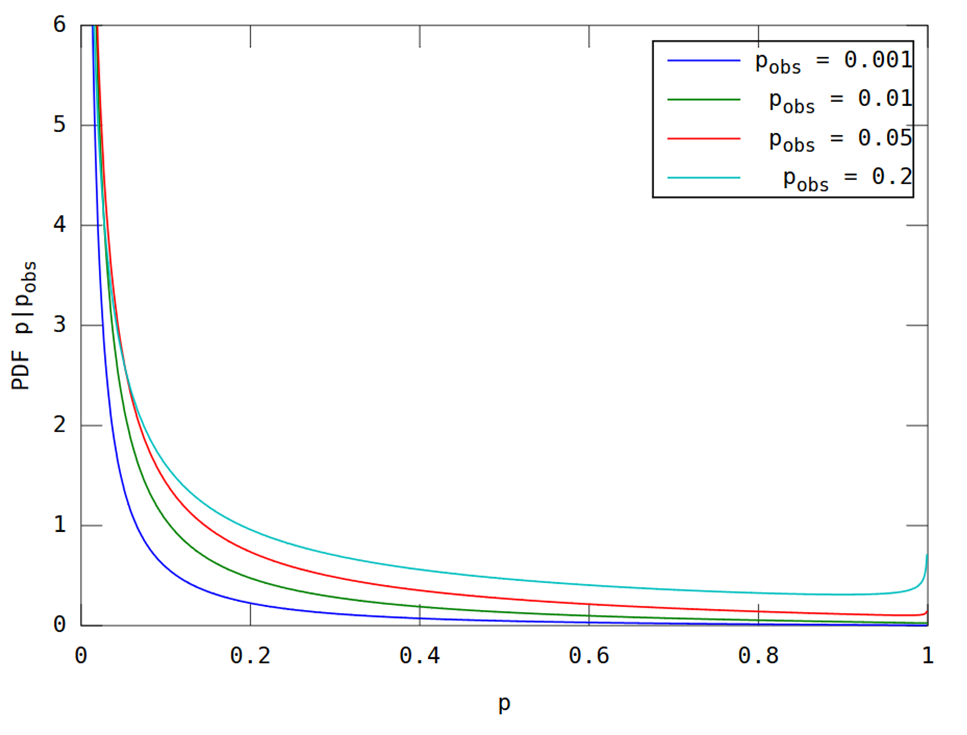
As requested in the comments, here is a plot for comparison. This is a relatively straightforward application of the formulas in the paper. However I will write these out to ensure no ambiguity.

Let $p$ denote the one-sided p value for the statistic $z$, and denote its (posterior) CDF by $F[u]\equiv\Pr\big[\,p\leq{u}\mid{\hat{z}}\,\big]$. Then equation B3 from the appendix is equivalent to $$F[p]=1-\Phi\left[\tfrac{1}{\sqrt{2}}\left(z[p]-\hat{z}\right)\right] \,,\, z[p]=\Phi^{-1}[1-p]$$ where $\Phi[\,\,]$ is the standard normal CDF. The corresponding density is then $$f\big[p\big]\equiv{F^\prime}\big[p\big]=\frac{\phi\Big[(z-\hat{z})/\sqrt{2}\,\Big]}{\sqrt{2}\,\phi\big[z\big]}$$ where $\phi[\,\,]$ is the standard normal PDF, and $z=z[p]$ as in the CDF formula. Finally, if we denote by $\hat{p}$ the observed two-sided p value corresponding to $\hat{z}$, then we have $$\hat{z}=\Phi^{-1}\Big[1-\tfrac{\hat{p}}{2}\Big]$$

Using these equations gives the figure below, which should be comparable to the paper's figure 5 quoted in the question.

(This was produced by the following Matlab code; run here.)

phat2=[1e-3,1e-2,5e-2,0.2]'; zhat=norminv(1-phat2/2);
np=1e3+1; p1=(1:np)/(np+1); z=norminv(1-p1);
p1pdf=normpdf((z-zhat)/sqrt(2))./(sqrt(2)*normpdf(z));
plot(p1,p1pdf,'LineWidth',1); axis([0,1,0,6]);
xlabel('p'); ylabel('PDF p|p_{obs}');
legend(arrayfun(@(p)sprintf('p_{obs} = %g',p),phat2,'uni',0));

Answer 2

Thanks for all the interesting discussions! When writing that 2008 article, it took me a while to convince myself that the distribution of replication p (the p value given by an exact replication of a study, meaning a study that is exactly the same, but with a new sample) is dependent only on p given by the original study. (In the paper I assume a normally distributed population and random sampling, and that our studies aim to estimate the mean of the population.) Therefore the p interval (the 80% prediction interval for replication p) is the same, whatever the N, power, or true effect size of the original study.

Sure, that's at first unbelievable. But note carefully that my original statement is based on knowing p from the original study. Think of it this way. Suppose you tell me that your original study has found p=.05. You tell me nothing else about the study. I know that the 95% CI on your sample mean extends exactly to zero (assuming p was calculated for a null hypothesis of zero). So your sample mean is MoE (the length of one arm of that 95% CI), because it is that distance from zero. The sampling distribution of means from studies like yours has standard deviation MoE/1.96. That's the standard error.

Consider the mean given by an exact replication. The distribution of that replication mean has mean MoE, i.e. that distribution is centred on your original sample mean. Consider the difference between your sample mean and a replication mean. It has variance equal to the sum of the variances of the mean of studies like your original study, and replications. That's twice the variance of studies like your original study, i.e. 2 x SE^2. Which is 2 x (MoE/1.96)^2. So the SD of that difference is SQRT(2) x MoE/1.96.

We therefore know the distribution of the replication mean: its mean is MoE and it's SD is SQRT(2) x MoE/1.96. Sure, the horizontal scale is arbitrary, but we only need to know this distribution in relation to the CI from your original study. As replications are run, most of the means (around 83%) will fall in that original 95% CI, and around 8% will fall below it (i.e. below zero, if your original mean was >0) and 8% higher than that CI. If we know where a replication mean falls in relation to your original CI, we can calculate its p value. We know the distribution of such replication means (in relation to your CI) so we can figure out the distribution of the replication p value. The only assumption we are making about the replication is that it is exact, i.e. it came from the same population, with the same effect size, as your original study, and that N (and the experimental design) was the same as in your study.

All the above is just a restating of the argument in the article, without pictures.

Still informally, it may be helpful to think what p=.05 in the original study implies. It could mean that you have an enormous study with a tiny effect size, or a tiny study with a giant effect size. Either way, if you repeat that study (same N, same population) then you will no doubt get a somewhat different sample mean. It turns out that, in terms of the p value, 'somewhat different' is the same, whether you had the enormous or the tiny study. So, tell me only your p value and I'll tell you your p interval.

Geoff

Answer 3

The issue has been clarified by @GeoMatt22, and I've been delighted to see @GeoffCumming coming here to participate in the discussion. I am posting this answer as a further commentary.

---

As it turns out, this discussion goes back at least to Goodman (1992) A comment on replication, P‐values and evidence and a later reply Senn (2002) Letter to the Editor. I can highly recommend reading these two brief articles, in particularly the Stephen Senn's one; I find myself fully agreeing with Senn.

If I had read these papers before asking this question, I would most likely have never posted it. Goodman (unlike Cumming) states very clearly that he considers a Bayesian setting with a flat prior. He does not present $p$-value distributions as Cumming does, and instead reports probabilities of observing a "significant" $p<0.05$ result in a replication experiment:

His main point is that these probabilities are surprisingly low (even for $p=0.001$ it is only $0.78$). In particular, for $p=0.05$ it is only $0.5$. (This latter $1/2$ probability remains the same for any $\alpha$ and $p=\alpha$.)

The point of Senn's reply is that this is a useful observation which, however, does not undermine $p$-values in any way and does not, contrary to Goodman, mean that $p$-values "overstate the evidence against the null". He writes:

I also consider that his [Goodman's] demonstration is useful for two reasons. First, it serves as a warning for anybody planning a further similar study to one just completed (and which has a marginally significant result) that this may not be matched in the second study. Second, it serves as a warning that apparent inconsistency in results from individual studies may be expected to be common and that one should not overreact to this phenomenon.

Senn reminds us that one-sided $p$-values can be understood as Bayesian posterior probabilities of $H_0:\mu<0$ under the flat prior for $\mu$ (improper prior on the whole real line) [see Marsman & Wagenmakers 2016 for a brief discussion of this fact and some citations].

If so, then having obtained any particular $p$-value in one experiment, probability that the next experiment will yield a lower $p$-value has to be $1/2$; otherwise future replications could somehow provide additional evidence before being conducted. So it makes total sense that for $p=0.05$ Goodman obtained probability $0.5$. And indeed, all replication distributions computed by Cumming and @GeoMatt22 have medians at the respective $p_\mathrm{obs}$.

We do not, however, need this replication probability to be higher than $0.5$ to believe that the efficacy of the treatment is probable. A long series of trials, $50$ per cent of which were significant at the $5$ per cent level, would be convincing evidence that the treatment was effective.

Incidentally, anybody who looked at the predictive distributions of $p$-values for, say, a t-test of given size and power (see e.g. here) will not be surprised that requiring a median at $p=0.05$ will necessarily make this distribution pretty broad, with a fat tail going towards $1$. In this light, broad intervals reported by Cumming cease being surprising.

What they rather do suggest, is that one should use larger sample sizes when trying to replicate an experiment; and indeed, this is a standard recommendation for replication studies (e.g. Uri Simonsohn suggests, as a rule of thumb, to increase sample size $2.5$-fold).

Answer 4

Thanks everyone for further interesting discussion. Rather than making my comments, point by point, I’ll offer some general reflections.

Bayes. I have nothing at all against Bayesian approaches. From the beginning I’ve expected that a Bayesian analysis, assuming a flat or diffuse prior, would give the same or very similar prediction intervals. There is a para on p. 291 in the 2008 article about that, partly prompted by one of the reviewers. So I’m pleased to see, above, a working through of that approach. That’s great, but it’s a very different approach from the one I took.

As an aside, I have chosen to work on advocacy of confidence intervals (the new statistics: effect sizes, CIs, meta-analysis) rather than Bayesian approaches to estimation (based on credible intervals) because I don’t know how to explain the Bayesian approaches to beginners sufficiently well. I haven’t seen any truly introductory Bayesian textbook that I feel I could use with beginners, or that is likely to be found accessible and convincing by large numbers of researchers. Therefore, we need to look elsewhere if we want to have a decent chance of improving the way researchers do their statistical inference. Yes, we need to move beyond p values, and shift from dichotomous decision making to estimation, and Bayesians can do that. But much more likely to achieve practical change, imho, is a conventional CI approach. That’s why our intro statistics textbook, recently released, takes the new statistics approach. See www.thenewstatistics.com

Back to reflections. Central to my analysis is what I mean by knowing only the p value from the first study. The assumptions I make are stated (normal population, random sampling, known population SD so we can use z rather than t calculations as we conduct inference about the population mean, exact replication). But that’s all I’m assuming. My question is ‘given only p from the initial experiment, how far can we go?’ My conclusion is that we can find the distribution of p expected from a replication experiment. From that distribution we can derive p intervals, or any probability of interest, such as the probability that the replication will give p<.05, or any other value of interest.

The core of the argument, and perhaps the step worth most reflection, is illustrated in Figure A2 in the article. The lower half is probably unproblematic. If we know mu (usually achieved by assuming it equals the mean from the initial study) then the estimation errors, represented by the thick line segments, have a known distribution (normal, mean mu, SD as explained in the caption).

Then the big step: Consider the upper half of Figure 2A. We have NO information about mu. No information—not any hidden assumption about a prior. Yet we can state the distribution of those thick line segments: normal, mean zero, SD = SQRT(2) times the SD in the lower half. That gives us what we need to find the distribution of replication p.

The resulting p intervals are astonishingly long—at least I feel astonishment when I compare with the way p values are virtually universally used by researchers. Researchers typically obsess about the second or third decimal place of a p value, without appreciating that the value they are seeing could very easily have been very different indeed. Hence my comments on pp 293-4 about reporting p intervals to acknowledge the vagueness of p.

Long, yes, but that doesn’t mean that p from the initial experiment means nothing. After a very low initial p, replications will tend, on average, to have smallish p values. Higher initial p and replications will tend to have somewhat larger p values. See Table 1 on p. 292 and compare, for example, the p intervals in the right column for initial p = .001 and .1—two results conventionally considered to be miles apart. The two p intervals are definitely different, but there is enormous overlap of the two. Replication of the .001 experiment could fairly easily give p larger than a replication of the .1 experiment. Although, most likely, it wouldn’t.

As part of his PhD research, Jerry Lai, reported (Lai, et al., 2011) several nice studies that found that published researchers from a number of disciplines have subjective p intervals that are far too short. In other words, researchers tend to under-estimate drastically how different the p value of a replication is likely to be.

My conclusion is that we should simply not use p values at all. Report and discuss the 95% CI, which conveys all the information in the data that tells us about the population mean we are investigating. Given the CI, the p value adds nothing, and is likely to suggest, wrongly, some degree of certainty (Significant! Not significant! The effect exists! It doesn’t!). Sure, CIs and p values are based on the same theory, and we can convert from one to the other (there’s lots on that in Chapter 6 of our intro textbook). But the CI gives way more information than p. Most importantly, it makes salient the extent of uncertainty. Given our human tendency to grasp for certainty, the extent of the CI is vital to consider.

I’ve also attempted to highlight the variability of p values in the ‘dance of the p values’ videos. Google ‘dance of the p values’. There are at least a couple of versions.

May all your confidence intervals be short!

Geoff