Strictly proper scoring rules are optimized in expected value by the true probabilities.
More informally, optimizing strictly proper scoring rules leads to your model seeking out the true probabilities. This sounds like the exact goal you have: to make probabilistic predictions as close to the true default probabilities as your can.
Two common strictly proper scoring rules are log loss and Brier score. Below, $y=(y_1,\dots,y_n)$ denotes the true observations $(y_i\in\{0, 1\})$, and $p = (p_1,\dots,p_n)$ denotes the predicted probabilities from a model $(p_i\in[0, 1])$.
$$
\text{Log Loss}\\
L(y, p) = -\dfrac{1}{n}\overset{n}{\underset{i=1}{\sum}}\bigg(
y_i\log(p_i) + (1-y_i)\log(1 - p_i)
\bigg)\\
\text{Brier Score}\\
B(y, p) = \dfrac{1}{n}\overset{n}{\underset{i=1}{\sum}}\bigg(
y_i - p_i
\bigg)^2
$$
A complaint about either of these might be that there is no sense of how good a score is, while a typical regression metric of $R^2$ gives a sense of model quality. First, that interpretation of $R^2$ is not as easy as one might hope, so I challenge the idea that any performance metric can be evaluated as "good" or "bad" without a context the way one might like to consider $90\%$ an $\text{A}$ in school while $40\%$ is an $\text{F}$. Second, both Brier score and log loss can be transformed to give $R^2$-style measures of performance. Let $\bar y$ be the proportion of $1$s in your data. Then McFadden's and Efron's pseudo $R^2$ values are defined as follows:
\overset{n}{\underset{i=1}{\sum}}\bigg(
y_i\log(p_i) + (1-y_i)\log(1 - p_i)
\bigg)
$$
R^2_{\text{McFadden}} = 1 - \left(\dfrac{
\overset{n}{\underset{i=1}{\sum}}\bigg(
y_i\log(p_i) + (1-y_i)\log(1 - p_i)
\bigg)
}{
\overset{n}{\underset{i=1}{\sum}}\bigg(
y_i\log(\bar y) + (1-y_i)\log(1 - \bar y)
\bigg)
}\right)
\\
R^2_{\text{Efron}} = 1 - \left(\dfrac{
\overset{n}{\underset{i=1}{\sum}}\bigg(
y_i - p_i
\bigg)^2
}{
\overset{n}{\underset{i=1}{\sum}}\bigg(
y_i - \bar y
\bigg)^2
}\right)
$$
As the $\bar y$ can be seen as the prior probability of a default, these pseudo $R^2$ values can be seen as comparisons of the values of strictly proper scoring rules achieved by the model compared to the value of that same strictly proper scoring rule that is achieved by predicting the prior probability every time, which is analogous to how the usual $R^2$ can be seen as comparing model predictions of the conditional mean to a model predicting the conditional mean as the marginal mean every time. Think about it this way: if you knew nothing about how your features influenced default probability, what would be your best guess for someone's default default probability if you knew the overall default rate to be $\bar y?$ These pseudo $R^2$ calculations go with the logic that the best naïve approach is to predict $\bar y$ every time.
If you want to do out-of-sample assessments of performance, I have a strong opinion about how to do that, a stance that now has support in the statistics literature from Hawinkel & Waegeman (2023)!
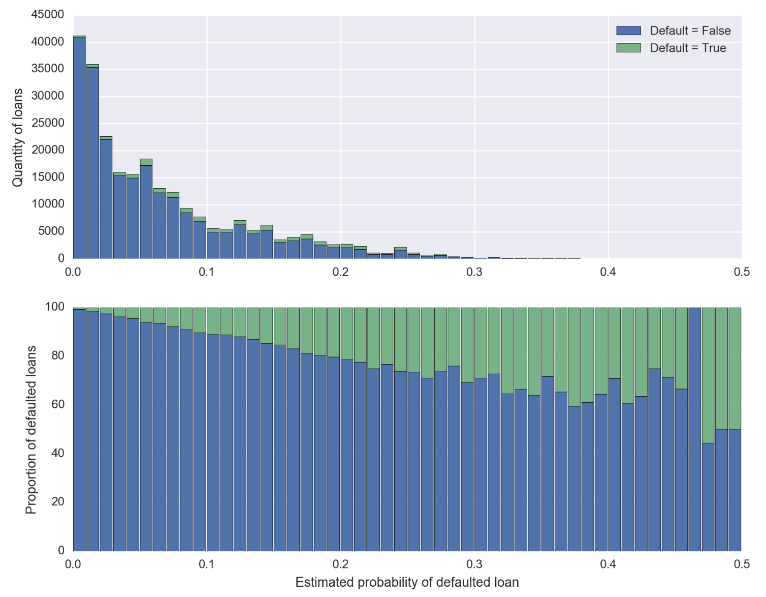
Finally, if you are checking that loans predicted to default with probabilities between $20\%$ and $30\%$ do default with the claimed probability, you are assessing your model calibration. I think the sklearn documentation gives a good idea of what this means and gives some references. What you are doing by binning into an interval like $[0.2, 0.3]$ is evocative of the Hosmer-Lemeshow test, which Frank Harrell argues is obsolete and replaced by techniques like those present in the sklearn function or his rms package (such as rms:calibrate).
I have a few posts on here about probability calibration.
Probability Calibration of Statistical Models
Should I use statistical tests (e.g., Hosmer-Lemeshow) to assess predictive models?
classification ML model: probability of positive label knowing the model score
Walk through rms::calibrate for logistic regression
Walk through rms::val.prob
REFERENCE
Hawinkel, Stijn, Willem Waegeman, and Steven Maere. "Out-of-sample R 2: estimation and inference." The American Statistician just-accepted (2023): 1-16.

