What is the distribution of the error around logistic growth data?

Question

In ecology, we often use the logistic growth equation:

$$ N_t = \frac{ K N_0 e^{rt} }{K + N_0 e^{rt-1}} $$

or

$$ N_t = \frac{ K N_0}{N_0 + (K -N_0)e^{-rt}} $$

where $K$ is the carrying capacity (maximum density reached), $N_0$ is the initial density, $r$ is the growth rate, $t$ is time since initial.

The value of $N_t$ has a soft upper bound $(K)$ and a lower bound $(N_0)$, with a strong lower bound at $0$.

Furthermore, in my specific context, measurements of $N_t$ are done using optical density or fluorescence, both of which have a theoretical maxima, and thus a strong upper bound.

The error around $N_t$ is thus probably best described by a bounded distribution.

At small values of $N_t$, the distribution probably has a strong positive skew, while at values of $N_t$ approaching K, the distribution probably has a strong negative skew. The distribution thus probably has a shape parameter that can be linked to $N_t$.

The variance may also increase with $N_t$.

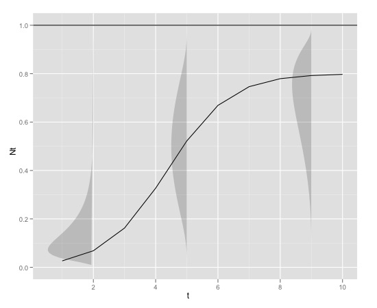
Here is a graphical example

with

K<-0.8
r<-1
N0<-0.01
t<-1:10
max<-1

which can be produced in r with

library(devtools)
source_url("https://raw.github.com/edielivon/Useful-R-functions/master/Growth%20curves/example%20plot.R")

• What would be the theoretical error distribution around $N_t$ (in consideration of both the model and the empirical information provided)?

• How doe the parameters of this distribution relate to the value of $N_t$ or time (if using parameters were the mode can not be directly associated with $N_t$ eg. logis normal)?

• Does this distribution have a density function implemented in $R$?

Directions explored so far:

• Assuming normality around $N_t$ (leads to over estimates of $K$)
• Logit normal distribution around $N_t/max$, but difficulty in fitting shape parameters alpha and beta
• Normal distribution around the logic of $N_t/max$

Answer 1

As Michael Chernick pointed out, the scaled beta distribution makes the best sense for this. However, for all practical purposes, and expecting that you will NEVER get the model perfectly right, you would be better off just modeling the mean via nonlinear regression according to your logistic growth equation and wrapping this up with standard errors that are robust to heteroskedasticity. Putting this into maximum likelihood context will create a false feeling of great accuracy. If the ecological theory would produce a distribution, you should fit that distribution. If your theory only produces the prediction for the mean, you should stick to this interpretation and don't try to come up with anything more than that, like a full-blown distribution. (Pearson's system of curves was surely fancy 100 years ago, but random processes do not follow differential equations to produce the density curves, which was his motivation with these density curves -- rather, one would think in terms of the central limit theorem as a way things may be working to produce distributions approximating what we see in practice.) I would expect that the variability goes up with the $N_t$ itself -- I am thinking of the Poisson distribution as an example -- and I am not entirely sure that this effect will be captured by the scaled beta distribution; it would, on the contrary, get compressed as you pull the mean towards its theoretical upper bound, which you may have to do. If your measurement device has an upper bound of the measurements, it does not mean that your actual process must have an upper bound; I would rather say that the measurement error introduced by your devices becomes critical as the process reaches that upper bound of being measured reasonably accurately. If you confound the measurement with the underlying process, you should recognize that explicitly, but I would imagine you have a greater interest in the process than in describing how your device works. (The process will be there 10 years from now; new measurement devices may become available, so your work will become obsolete.)

Answer 2

@whuber is correct that there is no necessary relationship of the structural part of this model to the distribution of error terms. So there is no answer to your question for the theoretical error distribution.

This doesn't mean that it isn't a good question though - just that the answer will have to be largely empirical.

You seem to be assuming that the randomness is additive. I see no reason (other than computational convenience) for this to be the case. Is an alternative that there is a random element somewhere else in the model? For example see the following, where randomness is introduced as Normally distributed with mean of 1, variance the only thing to estimate. I have no reason for thinking this is the right thing to do other than that it produces plausible results that seem to match what you want to see. Whether it would be practical to use something like this as the basis for estimating a model I don't know.

loggrowth <- function(K, N, r, time, rand=1){
    K*N*exp(rand*r*time)/(K+N*exp(rand*r*time-1)))}

plot(1:100, loggrowth(100,20,.08,1:100, rnorm(100,1,0.1)), 
    type="p", ylab="", xlab="time")
lines(1:100, loggrowth(100,20,.08,1:100))