Why linear regression has assumption on residual but generalized linear model has assumptions on response?

Question

Why linear regression and Generalized Model have inconsistent assumptions?

• In linear regression, we assume residual comes form Gaussian
• In other regression (logistic regression, poison regression), we assume response comes form some distribution (binomial, poission etc.).

Why sometimes assume residual and other time assume on response? Is is because we want to derive different properties?

---

EDIT: I think mark999's shows two forms are equal. However, I do have one additional doubts on i.i.d:

My other quesiton, Is there i.i.d. assumption on logistic regression? shows generalized linear model does not have i.i.d assumption (independent but not identical)

Is that true that for linear regression, if we pose assumption on residual, we will have i.i.d, but if we pose assumption on response, we will have independent but not identical samples (different Gaussian with different $\mu$)?

Answer 1

Simple linear regression having Gaussian errors is a very nice attribute that does not generalize to generalized linear models.

In generalized linear models, the response follows some given distribution given the mean. Linear regression follows this pattern; if we have

$y_i = \beta_0 + \beta_1 x_i + \epsilon_i$

with $\epsilon_i \sim N(0, \sigma)$

then we also have

$y_i \sim N(\beta_0 + \beta_1 x_i, \sigma)$

Okay, so the response follows the given distribution for generalized linear models, but for linear regression we also have that the residuals follow a Gaussian distribution. Why is it emphasized that the residuals are normal when that's not the generalized rule? Well, because it's the much more useful rule. The nice thing about thinking about normality of the residuals is this is much easier to examine. If we subtract out the estimated means, all the residuals should have roughly the same variance and roughly the same mean (0) and will be roughly normally distributed (note: I say "roughly" because if we don't have perfect estimates of the regression parameters, which of course we do not, the variance of the estimates of $\epsilon_i$ will have different variances based on the ranges of $x$. But hopefully there's enough precision in the estimates that this is ignorable!).

On the other hand, looking at the unadjusted $y_i$'s, we can't really tell if they are normal if they all have different means. For example, consider the following model:

$y_i = 0 + 2 \times x_i + \epsilon_i$

with $\epsilon_i \sim N(0, 0.2)$ and $x_i \sim \text{Bernoulli}(p = 0.5)$

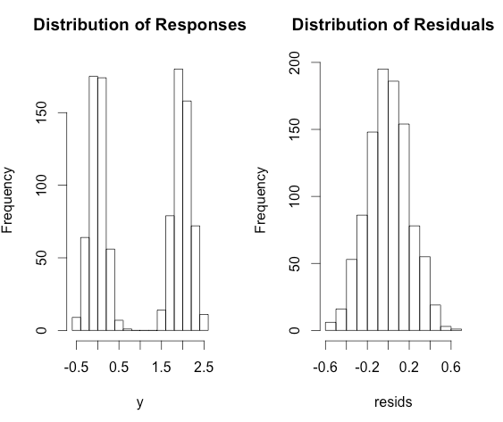
Then the $y_i$ will be highly bimodal, but does not violate the assumptions of linear regression! On the other hand, the residuals will follow a roughly normal distribution.

Here's some R code to illustrate.

x <- rbinom(1000, size = 1, prob = 0.5)
y <- 2 * x + rnorm(1000, sd = 0.2)
fit <- lm(y ~ x)
resids <- residuals(fit)
par(mfrow = c(1,2))
hist(y, main = 'Distribution of Responses')
hist(resids, main = 'Distribution of Residuals')

Answer 2

The assumptions are not inconsistent. If, for $i = 1, \ldots, n$, you assume $$ Y_i = \beta_0 + \beta_1 X_{i1} + \ldots + \beta_k X_{ik} + \epsilon_i, $$ with the errors $\epsilon_i$ being normally distributed with mean 0 and variance $\sigma^2$, that's the same as assuming that conditional on $X_{i1}, \ldots, X_{ik}$, the response $Y_i$ is normally distributed with mean $\beta_0 + \beta_1 X_{i1} + \ldots + \beta_k X_{ik}$ and variance $\sigma^2$.

This is because having conditioned on $X_{i1}, \ldots, X_{ik}$, we treat $\beta_0 + \beta_1 X_{i1} + \ldots + \beta_k X_{ik}$ as being constant.

The usual multiple linear regression model with normal errors is a generalised linear model with normal response and identity link.