Scikit correct way to calibrate classifiers with CalibratedClassifierCV

Question

Scikit has CalibratedClassifierCV, which allows us to calibrate our models on a particular X, y pair. It also states clearly that data for fitting the classifier and for calibrating it must be disjoint.

If they must be disjoint, is it legitimate to train the classifier with the following?

model = CalibratedClassifierCV(my_classifier)
model.fit(X_train, y_train)

I fear that by using the same training set I'm breaking the disjoint data rule. An alternative might be to have a validation set

my_classifier.fit(X_train, y_train)
model = CalibratedClassifierCV(my_classifier, cv='prefit')
model.fit(X_valid, y_valid)

Which has the disadvantage of leaving less data for training. Also, if CalibratedClassifierCV should only be fit on models fit on a different training set, why would it's default options be cv=3, which will also fit the base estimator? Does the cross validation handle the disjoint rule on its own?

Question: what is the correct way to use CalibratedClassifierCV?

Answer 1

There are two things mentioned in the CalibratedClassifierCV docs that hint towards the ways it can be used:

base_estimator: If cv=prefit, the classifier must have been fit already on data.

cv: If “prefit” is passed, it is assumed that base_estimator has been fitted already and all data is used for calibration.

I may obviously be interpreting this wrong, but it appears you can use the CCCV (short for CalibratedClassifierCV) in two ways:

Number one:

• You train your model as usual, your_model.fit(X_train, y_train).
• Then, you create your CCCV instance, your_cccv = CalibratedClassifierCV(your_model, cv='prefit'). Notice you set cv to flag that your model has already been fit.
• Finally, you call your_cccv.fit(X_validation, y_validation). This validation data is used solely for calibration purposes.

Number two:

• You have a new, untrained model.
• Then you create your_cccv=CalibratedClassifierCV(your_untrained_model, cv=3). Notice cv is now the number of folds.
• Finally, you call your_cccv.fit(X, y). Because your model is untrained, X and y have to be used for both training and calibration. The way to ensure the data is 'disjoint' is cross validation: for any given fold, CCCV will split X and y into your training and calibration data, so they do not overlap.

TLDR: Method one allows you to control what is used for training and for calibration. Method two uses cross validation to try and make the most out of your data for both purposes.

Answer 2

I am interested in this question as well and wanted to add some experiments to better understand CalibratedClassifierCV (CCCV).

As has already been said, there are two ways to use it.

#Method 1, train classifier within CCCV
model = CalibratedClassifierCV(my_clf)
model.fit(X_train_val, y_train_val)

#Method 2, train classifier and then use CCCV on DISJOINT set
my_clf.fit(X_train, y_train)
model = CalibratedClassifierCV(my_clf, cv='prefit')
model.fit(X_val, y_val)

Alternatively, we could try the second method but just calibrate on the same data we fitted on.

#Method 2 Non disjoint, train classifier on set, then use CCCV on SAME set used for training
my_clf.fit(X_train_val, y_train_val)
model = CalibratedClassifierCV(my_clf, cv='prefit')
model.fit(X_train_val, y_train_val)

Although the docs warn to use a disjoint set, this could be useful because it allows you to then inspect my_clf (e.g., to see the coef_, which are unavailable from the CalibratedClassifierCV object). (Does anyone know how to get this from the calibrated classifiers---for one, there are three of them so would you average coefficients?).

I decided to compare these 3 methods in terms of their calibration on a completely held out test set.

Here is a dataset:

X, y = datasets.make_classification(n_samples=500, n_features=200,
                                    n_informative=10, n_redundant=10,
                                    #random_state=42, 
                                    n_clusters_per_class=1, weights = [0.8,0.2])

I threw in some class imbalance and only provided 500 samples to make this a difficult problem.

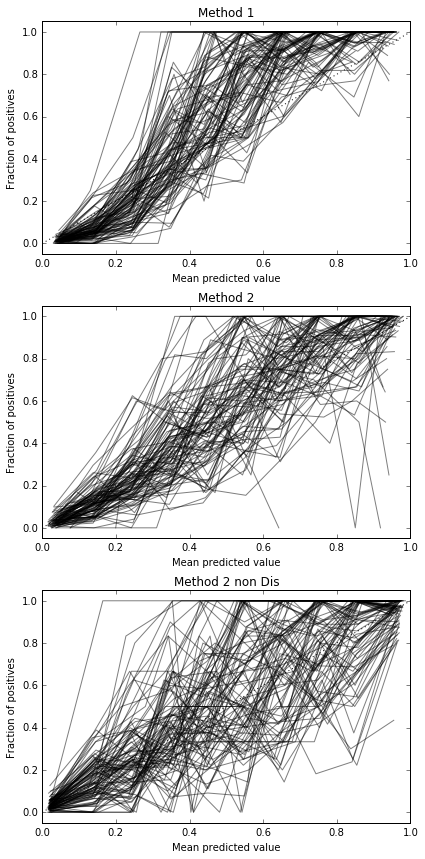
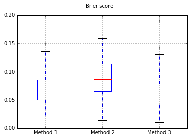
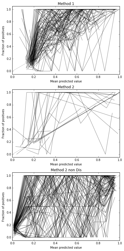
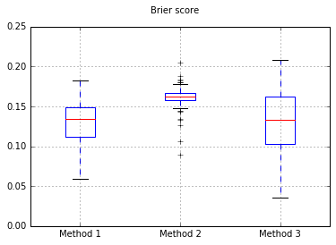
I run 100 trials, each time trying each method and plotting its calibration curve.

Boxplots of the Brier scores over all trials:

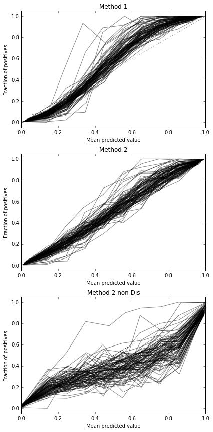
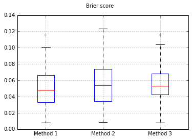
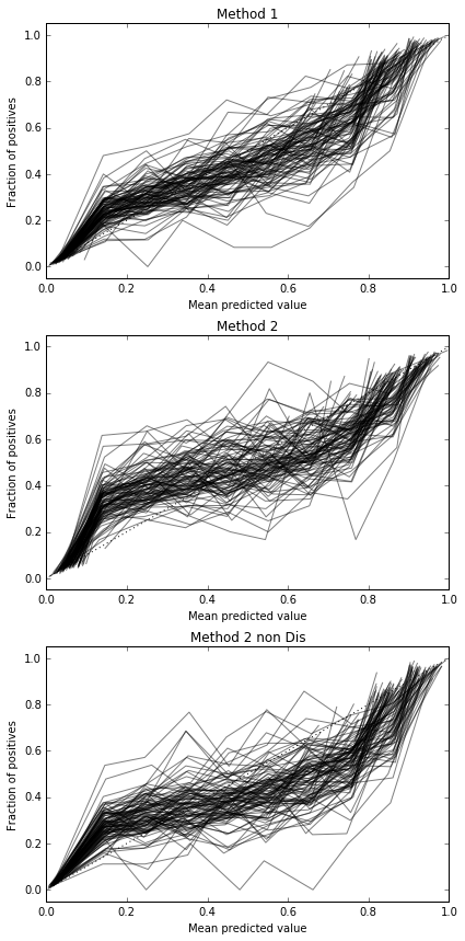
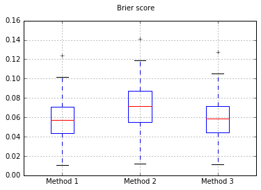
Increasing the number of samples to 10,000:

If we change the classifier to Naive Bayes, going back to 500 samples:

This appears not to be enough samples to calibrate. Increasing samples to 10,000

Full code

print(__doc__)

# Based on code by Alexandre Gramfort <[email protected]>
#         Jan Hendrik Metzen <[email protected]>

import matplotlib.pyplot as plt

from sklearn import datasets
from sklearn.naive_bayes import GaussianNB
from sklearn.linear_model import LogisticRegression
from sklearn.metrics import brier_score_loss
from sklearn.calibration import CalibratedClassifierCV, calibration_curve
from sklearn.model_selection import train_test_split


def plot_calibration_curve(clf, name, ax, X_test, y_test, title):

    y_pred = clf.predict(X_test)
    if hasattr(clf, "predict_proba"):
        prob_pos = clf.predict_proba(X_test)[:, 1]
    else:  # use decision function
        prob_pos = clf.decision_function(X_test)
        prob_pos = \
            (prob_pos - prob_pos.min()) / (prob_pos.max() - prob_pos.min())

    clf_score = brier_score_loss(y_test, prob_pos, pos_label=y.max())

    fraction_of_positives, mean_predicted_value = \
        calibration_curve(y_test, prob_pos, n_bins=10, normalize=False)

    ax.plot(mean_predicted_value, fraction_of_positives, "s-",
             label="%s (%1.3f)" % (name, clf_score), alpha=0.5, color='k', marker=None)

    ax.set_ylabel("Fraction of positives")
    ax.set_ylim([-0.05, 1.05])
    ax.set_title(title)

    ax.set_xlabel("Mean predicted value")

    plt.tight_layout()
    return clf_score

    fig, (ax1, ax2, ax3) = plt.subplots(nrows=3, ncols=1, figsize=(6,12))

    ax1.plot([0, 1], [0, 1], "k:", label="Perfectly calibrated",)
    ax2.plot([0, 1], [0, 1], "k:", label="Perfectly calibrated")
    ax3.plot([0, 1], [0, 1], "k:", label="Perfectly calibrated")

    scores = {'Method 1':[],'Method 2':[],'Method 3':[]}


fig, (ax1, ax2, ax3) = plt.subplots(nrows=3, ncols=1, figsize=(6,12))

ax1.plot([0, 1], [0, 1], "k:", label="Perfectly calibrated",)
ax2.plot([0, 1], [0, 1], "k:", label="Perfectly calibrated")
ax3.plot([0, 1], [0, 1], "k:", label="Perfectly calibrated")

scores = {'Method 1':[],'Method 2':[],'Method 3':[]}

for i in range(0,100):

    X, y = datasets.make_classification(n_samples=10000, n_features=200,
                                        n_informative=10, n_redundant=10,
                                        #random_state=42, 
                                        n_clusters_per_class=1, weights = [0.8,0.2])

    X_train_val, X_test, y_train_val, y_test = train_test_split(X, y, test_size=0.80,
                                                        #random_state=42
                                                               )

    X_train, X_val, y_train, y_val = train_test_split(X_train_val, y_train_val, test_size=0.80,
                                                      #random_state=42
                                                     )

    #my_clf = GaussianNB()
    my_clf = LogisticRegression()

    #Method 1, train classifier within CCCV
    model = CalibratedClassifierCV(my_clf)
    model.fit(X_train_val, y_train_val)
    r = plot_calibration_curve(model, "all_cal", ax1, X_test, y_test, "Method 1")
    scores['Method 1'].append(r)

    #Method 2, train classifier and then use CCCV on DISJOINT set
    my_clf.fit(X_train, y_train)
    model = CalibratedClassifierCV(my_clf, cv='prefit')
    model.fit(X_val, y_val)
    r = plot_calibration_curve(model, "all_cal", ax2, X_test, y_test, "Method 2")
    scores['Method 2'].append(r)

    #Method 3, train classifier on set, then use CCCV on SAME set used for training
    my_clf.fit(X_train_val, y_train_val)
    model = CalibratedClassifierCV(my_clf, cv='prefit')
    model.fit(X_train_val, y_train_val)
    r = plot_calibration_curve(model, "all_cal", ax3, X_test, y_test, "Method 2 non Dis")
    scores['Method 3'].append(r)

import pandas
b = pandas.DataFrame(scores).boxplot()
plt.suptitle('Brier score')

So, the Brier score results are inconclusive, but according to the curves it seems to be best to use the second method.