Over-represented values in FDR-adjusted p-values

Question

I have a vector of p-values that need correcting for multiple comparisons; based on reading Noble (2009), I am attempting to apply a Benjamini-Hochberg FDR-based correction.

My vector (sorted in ascending order for ease of visualisation) is:

ps <- c(0.019, 0.022, 0.023, 0.023, 0.025, 0.025, 0.027, 0.028, 0.029, 0.030, 0.030, 0.030, 0.031, 0.033, 0.034, 0.035, 0.036, 0.037, 0.037, 0.039, 0.051, 0.060, 0.063, 0.065, 0.085, 0.110, 0.170, 0.196, 0.241, 0.316, 0.318, 0.325, 0.694)

When I run the R commmand

p.adjust(ps, method="BH")

I get the output:
0.06426316 0.06426316 0.06426316 0.06426316 0.06426316 0.06426316 0.06426316 0.06426316 0.06426316 0.06426316 0.06426316 0.06426316 0.06426316 0.06426316 0.06426316 0.06426316 0.06426316 0.06426316 0.06426316 0.06435000 0.08014286 0.08937500 0.08937500 0.08937500 0.11220000 0.13961538 0.20777778 0.23100000 0.27424138 0.33515625 0.33515625 0.33515625 0.69400000

This output clearly has certain values that are over-represented. Given that they are the same to 8 decimal places, I don't think it is likely to happen by chance. If I plot the raw and adjusted values, they both follow the same topography but the adjusted values plateau whenever the raw values have a small slope.

plot(ps~order(ps))
points(p.adjust(ps, method="BH")~order(ps), add=TRUE, col="red")

Generally, it seems that when a raw p-value has a difference <0.01 from the next-highest value, the corrected values come out identical. I can't understand why, though; I've read around and dug into the p.adjust code, but can't think what would cause this effect. Any insight would be greatly appreciated!

Answer 1

There is nothing wrong with these q-values. Correcting p-values (corrected p-values are often referred to as q-values) is a concept that's newer than the Benjamini-Hochberg (BH) procedure, which in its purest form only outputs significant: yes or no. To understand why your q-values look the way they look we need to look at how the BH step-up procedure works. The steps below are adapted from Wasserman's All of Statistics:

1. Order your p-values $p_1 < p_2 < \ldots < p_m$.
2. Define $l_i = \frac{i\alpha}{m}$, where $\alpha$ is your desired false discovery rate. Also define $T = \max\{p_i: p_i < l_i\}$, ie $T$ is the largest p-value for which $p_i < l_i$.
3. Let $T$ be your BH rejection threshold.
4. Reject the null-hypotheses $H_{0i}$ for which $p_i \leq T$.

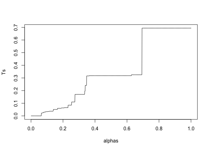
To avoid having to choose an $\alpha,$ the q-value turns this procedure upside-down and asks what is the smallest $\alpha$ at which $H_{0i}$ would be rejected? The threshold $T$ is always going to be one of your $m$ p-values, so the threshold for acceptance as a function of the FDR $\alpha$ is going to look like some stairs:

library(plyr)
ps <- c(0.019, 0.022, 0.023, 0.023, 0.025, 0.025, 0.027, 0.028, 0.029, 0.030, 0.030, 0.030, 0.031, 0.033, 0.034, 0.035, 0.036, 0.037, 0.037, 0.039, 0.051, 0.060, 0.063, 0.065, 0.085, 0.110, 0.170, 0.196, 0.241, 0.316, 0.318, 0.325, 0.694)

# calculate T as function of alpha
BHT <- function(alpha) {
  l <- 1:length(ps)*alpha/length(ps)
  i <- sum(ps < l)
  if (i == 0) return(i)

  ps[i]   # threshold
}

alphas <- seq(0,1,by=.001)
Ts <- aaply(alphas, 1, BHT)
plot(alphas, Ts, type="l")

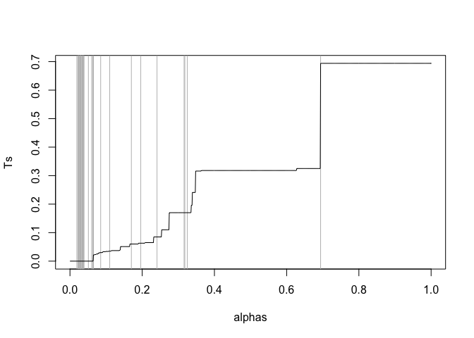
For each threshold, there is a single smallest $\alpha$ that makes this the new rejection threshold. If we put some lines in the previous plot for your different p-values, you'll see that many of them sit on the same step of the staircase:

plot(alphas, Ts, type="n")
abline(v=ps, col="grey")
lines(alphas, Ts)

These will get rejected at the same threshold and correspond to the same smallest $\alpha$. This $\alpha$ is your q-value, so it's OK and pretty much inevitable to get repeated q-values.