Confidence Interval (CI) calculation of Monte Carlo-simulated non-normal data

Question

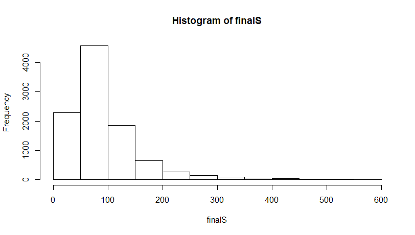
I’m trying to identify the 95% confidence interval of either the mean or the median of non-normal data generated through Monte Carlo simulations using R. I’ve already applied both the bootstrapping method as well as the Wilcoxon signed rank test as suggested on the following thread: How do I calculate confidence intervals for a non-normal distribution?. However the resulting CIs from both tests seem suspiciously small, especially given the overall spread of the data .

#Install truncdist - to truncate distributions
install.packages("truncdist")
library(truncdist)

#Monte Carlo simulations
S1 <- rtrunc(10000, spec = "lnorm",a=0, b=1600, meanlog=4.4166,sdlog=1.1334)
S2 <- rtrunc(10000, spec = "logis",a=0, location = 97.056, scale = 50.86)
S3 <- rtrunc(10000, spec = "norm", a=0, mean=11.3,sd=4.45)

#Calculate averages of Monte Carlo simulations
SampleS <- matrix(c(S1,S2,S3),nrow = 10000,ncol = 3)
finalSmeans <- rowMeans(SampleB)
hist(finalS)

#Install package to run bootstrap
install.packages("resample")
library(resample)

#Bootstrap CI for mean
bootmean <- bootstrap(finalS, mean, R=1000)
CI.bca(bootmean)
     2.5%   97.5%
mean 91.99672 94.8231

#Bootstrap CI for median
bootmedian <- bootstrap(finalS, median, R=1000)
CI.bca(bootmedian)
       2.5%    97.5%
median 74.54763 76.87361

#Wilcoxon test for median CIs
wilcox.test(finalS, conf.int = TRUE, conf.level = 0.95)

   Wilcoxon signed rank test with continuity correction

data:  finalS
V = 50005000, p-value < 2.2e-16
alternative hypothesis: true location is not equal to 0
95 percent confidence interval:
   80.58888 82.58312
sample estimates:
(pseudo)median 
   81.5794 

Have I done something wrong? Are these tests appropriate to use when evaluating distributions generated through Monte Carlo simulations? Or are there more robust tests out there that I'm not aware of?

Answer 1

It is not really clear what do you want to achieve and as already noted by Björn there is not reason why you should expect anything else then narrow confidence intervals with such large sample.

Since you are doing simulation, you can explicitly simulate the distribution of means (or medians) and verify that actually the bootstrap confidence interval quite closely covers the 95% quantile interval of the distribution of empirical means (see code example below).

simfun <- function() {
  S1 <- rtrunc(10000, spec = "lnorm",a=0, b=1600, meanlog=4.4166,sdlog=1.1334)
  S2 <- rtrunc(10000, spec = "logis",a=0, location = 97.056, scale = 50.86)
  S3 <- rtrunc(10000, spec = "norm", a=0, mean=11.3,sd=4.45)

  SampleS <- matrix(c(S1,S2,S3),nrow = 10000,ncol = 3)
  finalSmeans <- rowMeans(SampleS)
  mean(finalSmeans)
}

CI.bca(bootmean)
##          2.5%    97.5%
## mean 92.92275 95.62323
quantile(replicate(500, simfun()), c(0.025, 0.975)) 
##     2.5%    97.5% 
## 91.39106 94.13525