Inconsistency in statistics: parameters estimation with heteroskedasticity

Question

I want to estimate this model $$ y_t = a + b x_t + \sigma x_t\epsilon_t $$ where we have an error with heteroskedasticity (it depends on $x_t$).

Suppose I estimate this model with OLS so, assuming that the error is homoskedastic. In particular, I'am assuming that the model is $$ y_t = a + b x_t + \epsilon_t $$
with $\epsilon_t$ ~ $N(0,\eta^2)$. I get $\hat{a}, \hat{b}$ and a set of residuals $\hat{\epsilon}_t$.

Now I want to estimate $\sigma$. I can set up another regression $$ \log(\epsilon_t) = \log(\sigma)+\log(x_t)+\epsilon_t. $$ But it seems to me that there is an inconsistency in doing this. How can I do this correctly?

Answer 1

Your basic idea seems sound! You want to estimate a linear model with heteroskedasticity, but you don't know in which way the variance depends on the covariables, so you want to estimate that via a second model. That can be done, but to obtain correct results you must iterate the process, first estimate the linear model using constant variance, then estimate the model for the variance using residuals, then using the estimated variance model, going back and reiterating your first linear model, and so continuing, alternating both steps, until convergence.

But the particular way you set it up is incorrect. In particular, you take log of the residuals. That cannot work, because some of the residuals are bound to be negative! That's maybe the way you detected that something was fishy ...

To do this correctly, you can reformulate using generalized linear models, and link functions in place of data transformations. That process can be done, and is implemented for instance in R, in the package dglm, double generalized linear models. For an example of its use, see Simulate linear regression with heteroscedasticity or search this site for dglm, there are other examples!

Another possibility is the R package gamlss, look at the tag gamlss.

Answer 2

Note that in your last equation, you need a different symbol for the population noise term $y_t-a-bx_t$ than $\epsilon_t$ (i.e. the one on the LHS of your last equation) since $\epsilon_t$ is already used for something else. I suggest writing $y_t = a + bx_t + \eta_t$ where $\eta_t = \sigma x_t \epsilon_t$. [Note that you don't need $\eta$ for the variance of $\epsilon$ since it would be absorbed into $\sigma$; just make $\epsilon$ standard normal.]

However you can only take logs of that last equation if $\epsilon$, $\eta$ and $x$ are each always positive. That might be okay to assume for $x$ but it definitely doesn't make sense for $\epsilon$, since you already specified that it's $\leq 0$ half the time.

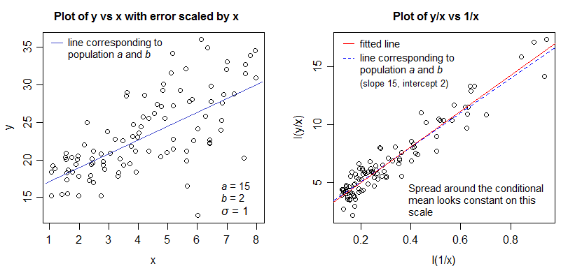
An alternative to consider is to divide the first equation through by $x_t$, giving $y^*_t = ax^*_t + b + \sigma\epsilon_t$ where $y^* = y/x$ and $x^*= 1/x$. It may be suitable in some circumstances.

With that transformation, this is now a constant-variance linear regression, but now $a$ and $b$ have swapped roles (that is, the slope in this equation is the intercept in the original and vice-versa).

A simulated example where it works well: