Approximation error of confidence interval for the mean when $n \geq 30$

Question

Let $\{X_i\}_{i=1}^n$ be a family of i.i.d. random variables taking values in $[0,1]$, having a mean $\mu$ and variance $\sigma^2$. A simple confidence interval for the mean, using $\sigma$ whenever it is known, is given by $$ P( | \bar X - \mu| > \varepsilon) \le \frac{\sigma^2}{n\varepsilon^2} \le\frac{1}{n \varepsilon^2} \qquad (1). $$

Also, because $\frac{\bar X- \mu}{\sigma/\sqrt{n}}$ is asymptotically distributed as a standard normal random variable, the normal distribution is sometimes used to "construct" an approximate confidence interval.

---

In multiple-choice answer statistics exams, I've had to use this approximation instead of $(1)$ whenever $n \geq 30$. I've always felt very uncomfortable with this (more than you can imagine), as the approximation error is not quantified.

---

• Why use the normal approximation rather than $(1)$?

• I don't want, ever again, to blindly apply the rule $n \geq 30$. Are there good references that can support me in a refusal to do so and provide appropriate alternatives? ($(1)$ is an example of what I consider an appropriate alternative.)

Here, while $\sigma$ and $E[ |X|^3]$ are unknown, they are easily bounded.

Please note that my question is a reference request particularly about confidence intervals and therefore is distinct from the differs from the questions that were suggested as partial duplicates here and here. It is not answered there.

Answer 1

Why use normal approximation?

It's as simple as saying that it's always better to use more information than less. The equation (1) uses Chebyshev's theorem. Note, how it doesn't use any information about your distribution's shape, i.e. it works for any distribution with a given variance. Hence, if you use some information about your distribution's shape you must get a better approximation. If you knew that your distribution is Gaussian, then by using this knowledge you get a better estimate.

Since, you're already applying the central limit theorem, why not use the Gaussian approximation of the bounds? They're going to be better, actually, tighter (or sharper) because these estimates are based on the knowledge of the shape which is an additional piece of information.

The rule of thumb 30 is a myth, which benefits from the confirmation bias. It just keeps being copied from one book to another. Once I found a reference suggesting this rule in a paper in 1950s. It wasn't any kind of solid proof, as I recall. It was some sort of empirical study. Basically, the only reason it's used is because it sort of works. You don't see it violated badly often.

UPDATE Look up the paper by Zachary R. Smith and Craig S. Wells "Central Limit Theorem and Sample Size". They present an empirical study of the convergence to CLT for different kinds of distributions. The magic number 30 doesn't work in many cases, of course.

Answer 2

The issue with using the Chebyshev inequality to obtain an interval for the true value, is that it only gives you a lower bound for the probability, which moreover is sometimes trivial, or, in order not to be trivial, it may give a very wide confidence interval. We have

$$P( | \bar X - \mu| > \varepsilon) = 1 - P(\bar X-\varepsilon \leq \mu \leq \bar X+\varepsilon)$$

$$\implies P(\bar X-\varepsilon \leq \mu \leq \bar X+\varepsilon) \geq 1- \frac{1}{n \varepsilon^2}$$

We see that, depending also on sample size, if we decrease $\varepsilon$ "too much" we will get the trivial answer "the probability is greater than zero".

Apart from that, what we get from this approach is a conclusion of the form ""the probability of $\mu$ falling in $[\bar X \pm \varepsilon]$ is equal or greater than..."

But let's assume that we're good with this, and denote $p_{min}$ the minimum probability with which we are comfortable. So we want

$$ 1- \frac{1}{n \varepsilon^2} = p_{min} \implies \varepsilon = \sqrt {\frac {1}{(1-p_{min})n}}$$

With small sample sizes and high desired minimum probability, this may give an unsatisfactorily wide confidence interval. E.g. for $p_{min} =0.9$ and $n=100$ we will get $\varepsilon \approx .316$, which, for example for the variable treated by the OP that is bounded in $[0,1]$ appears to be too big to be useful.

But the approach is valid, and distribution-free, and so there may be instances where it can be useful.

One may want to check also the Vysochanskij–Petunin inequality mentioned in another answer, which holds for continuous unimodal distributions and refines Chebyshev's inequality.

Answer 3

The short answer is that it can go pretty badly, but only if one or both tails of the sampling distribution is really fat.

This R code generate a million sets of 30 gamma-distributed variables and take their mean; it can be used to get a sense of what the sampling distribution of the mean looks like. If the normal approximation works as intended, the results should be approximately normal with mean 1 and variance 1/(30 * shape).

f = function(shape){replicate(1E6, mean(rgamma(30, shape, shape)))}

When shape is 1.0, the gamma distribution becomes an exponential distribution, which is pretty non-normal. Nevertheless, the non-Gaussian parts mostly average out and so Gaussian approximation isn't so bad:

There's clearly some bias, and it would be good to avoid that when possible. But honestly, that level of bias probably won't be the biggest problem facing a typical study.

That said, things can get much worse. With f(0.01), the histogram looks like this:

Log-transforming the 30 sampled data points before averaging helps a lot, though:

In general, distributions with long tails (on one or both sides of the distribution) will require the most samples before the Gaussian approximation starts to become reliable. There are even pathological cases where there will literally never be enough data for the Gaussian approximation to work, but you'll probably have more serious problems in that case (because the sampling distribution doesn't have a well-defined mean or variance to begin with).

Answer 4

Problem with the Chebyshev confidence interval

As mentioned by Carlo, we have $\sigma^2 \le \frac{1}{4}$. This follows from $\text{Var}(X) \le \mu(1-\mu)$. Therefore a confidence interval for $\mu$ is given by $$ P(|\bar{X}-\mu| \geq \varepsilon) \le \frac{1}{4n\varepsilon^2}. $$ The problem is that the inequality is, in a certain sense, quite loose when $n$ gets large. An improvement is given by Hoeffding's bound and shown below. However, we can also demonstrate how bad it can get using the Berry-Esseen theorem, pointed out by Yves. Let $X_i$ have a variance $\tfrac{1}{4}$, the worst possible case. The theorem implies that $ P(|\bar X - \mu| \geq \tfrac{\varepsilon}{2\sqrt{n}}) \le 2\, \text{SF}(\varepsilon) + \tfrac{8}{\sqrt{n}}, $ where $\text{SF}$ is the survival function of the standard normal distribution. In particular, with $\varepsilon = 16$, we get $\text{SF}(16) \approx e^{-58}$ (according to Scipy), so that essentially $$ P(|\bar X - \mu| \geq \tfrac{8}{\sqrt{n}}) \le \tfrac{8}{\sqrt{n}} + 0, \qquad (*) $$ whereas the Chebyshev inequality implies $$ P(|\bar X - \mu| \geq \tfrac{8}{\sqrt{n}}) \le \tfrac{1}{256}. $$ Note that I did not try to optimize the bound given in $(*)$, the result here is only of conceptual interest.

---

Comparing the lengths of the confidence intervals

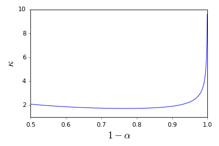
Consider the $(1-\alpha)$-level confidence interval lengths $\ell_Z(\alpha, n)$ and $\ell_C(\alpha, n)$ obtained using the normal approximation ($\sigma = \tfrac{1}{2}$) and the Chebyshev inequality, repectively. It turns out that $\ell_C(\alpha, n)$ is a constant times bigger than $\ell_Z(\alpha, n)$, independently of $n$. Precisely, for all $n$, $$ \ell_C(\alpha, n) = \kappa(\alpha) \ell_Z(\alpha, n), \quad \kappa(\alpha) = \left(\text{ISF}\left(\tfrac{\alpha}{2}\right) \sqrt{\alpha}\right)^{-1}, $$ where $\text{ISF}$ is the inverse survival function of the standard normal distribution. I plot below the multiplicative constant.

$\hskip 1in$

In particular, the $95\%$ level confidence interval obtained using the Chebyshev inequality is about $2.3$ times bigger than the same level confidence interval obtained using the normal approximation.

---

Using Hoeffding's bound

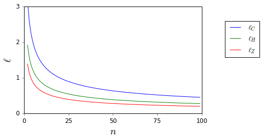
Hoeffding's bound gives $$ P(|\bar X - \mu| \geq \varepsilon) \leq 2e^{-2n \varepsilon^2}. $$ Thus an $(1-\alpha)$-level confidence interval for $\mu$ is $$ (\bar X - \varepsilon, \bar X + \varepsilon), \quad \varepsilon = \sqrt{\frac{-\ln \tfrac{\alpha}{2}}{2n}}, $$ of length $\ell_H (\alpha, n) = 2\varepsilon$. I plot below the lengths of the different confidence intervals (Chebyshev inequality: $\ell_C$; normal approximation ($\sigma = 1/2$): $\ell_Z$; Hoeffding's inequality: $\ell_H$) for $\alpha = 0.05$.

$\hskip 0.5in$

Answer 5

let's start with the number 30: it's, as anyone will say, a rule of thumb. but how can we find a number that fits better to our data? It's actually mostly a matter of skewness: even the strangest distribution will fast converge to normal if they are simmetric and continuous, skewed data will be much slower. I remember learning that a binomial distribution can be properly approximated to normal when its variance is greater than 9; for this example it's to be considered that discrete distribution also have the problem that they need great numbers to simulate continuity, but think to this: a simmetric binomial distribution will reach that variance with n = 36, if p = 0.1 instead, n must go up to 100 (variabile trasformation, however, would help a lot)!

If you only want to use variance instead, dropping gaussian approximation, consider Vysochanskij–Petunin inequality over Chebichev's, it needs the assumption of unimodal distribution of the mean, but this is a very safe one with any sample size, I'd say, greater than 2.