p-value for complete spatial randomness tests

Question

I am using the Kolmogorov-Smirnov test to study the homogeneity of a point pattern in 3D using the distance transform to a structure as a covariate.

I am using the spatstat book, where it is explained (Section 10.5) that the Kolmogorov-Smirnov test statistic ($D$) can be calculated as the maximum vertical separation between the cumulative distribution function of the spatial covariate evaluated at the data points ($F_0(z)$) and at all locations ($\hat{F}(z)$). It is:

$D = \max\limits_z|\hat{F}(z)-F_0(z)|$

However, I do not understand how to obtain the value $D$ for my null hypothesis (that the points are homogeneously distributed) so that I can compare them and know whether I can reject the null hypothesis.

If there is also a formula to calculate the critical p-value would be excellent, since I read how to calculate it when you compare your data with a defined distribution like Poisson, but in this case I understand that I should use $\hat{F}(z)$ as the distribution to compare.

Furthermore, I could only use this test in spatstat for 2D data, but not for 3D. If will also appreciate any hint about how to do it.

EDIT: Following the example in the spatstat book, what I am doing is:

elev <- bei.extra$elev
cdf.test(bei,elev)

Which produces this result:

Spatial Kolmogorov-Smirnov test of CSR in two dimensions

data:  covariate ‘elev’ evaluated at points of ‘bei’ 
     and transformed to uniform distribution under CSR
D = 0.10634, p-value < 2.2e-16
alternative hypothesis: two-sided

As far as I understand, $D$ is calculated with the formula above, however that says nothing about the rejection of the null hypothesis. Now I would like to know how the p-value can be calculated.

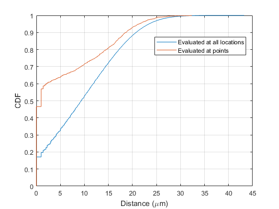
As I want to do this test in 3D data, I apply the distance transform in 3D to the structure of interest (covariate), and I compare its result evaluated at all locations $\hat{F}(z)$ and at the observed points ($F_0(z)$). Then, I can compare the distributions as in this figure:

At this point I know how to calculate $D$, but again, that does not tell if the null hypothesis can be rejected. In this figure it looks obvious that the the points are not homogeneously distributed, but I would like to calculate with which p-value I can reject the null hypothesis.

EDIT 2: Two-Sample Kolmogorov-Smirnov test. Up to now I have been using the two-sample Kolmogorov-Smirnov test as Ege Rubak mentioned in his answer. I was using the MATLAB function kstest2 that calculates the p-value based on the number of samples in $x$ (length(x)) and $y$ (length(y)), where $x$ is a vector with the data points and $y$ the covariate values at the grid points.

The problem is that the size of $y$ corresponds to the number of pixels in the image and are not ‘real’ samples. This means that if my image has a small pixel size or I use a smaller grid (independently of the real volume of the sample) it will be easier to reject the null hypothesis. As far as I understand (please correct me if I am wrong) the test should only consider the size of $x$, since it contains the real samples, and not length(y).

Now I was checking the R code that Ege Rubak proposed to understand what it is actually doing, and I found that the ks.test function calls the function psmirnov2x in C code (which I could not found). The inputs of this function are $D$ (maximum distance between CDFs), length(x) and length(y), so I understand that in this function the p-value is also based on the lengths of both vectors. Am I wrong thinking that this is not the correct approach? Or should I find a different way of doing this test?

Answer 1

The code in spatstat calls ks.test() which is a default R function (in stats package), so the actual calculation of the p-value under the null hypothesis is done there. In the spatstat code a few tricks are done (e.g. transformation to uniform distribution using the inverse CDF), so it might not be easy to follow that code. I see two different options:

1. Quick and dirty with two sample KS test.
2. Transform to uniform distribution and use one sample KS test.

Option 1

I think you can simply calculate the two sample KS test and get what you want. Simply put the covariate values at the data points in a vector x and the covariate values at the grid points in a vector y and then do ks.test(x,y). In principle the more grid points you can afford the better. As you add more grid points I expect the p-value converges to the optimal you can get from a two sample KS test. It may however still be different (probably conservative) than what the p-value a one sample KS test would give. Following the example from the book:

require(spatstat, quietly = TRUE)
#> 
#> spatstat 1.49-0.011       (nickname: 'Instinctively Correct') 
#> For an introduction to spatstat, type 'beginner'
# Covariate image
elev <- bei.extra$elev
# Data values:
x <- elev[bei]
# Grid values (simply extracted from image):
y <- as.matrix(elev)
# Test
test <- ks.test(x,y)
#> Warning in ks.test(x, y): p-value will be approximate in the presence of
#> ties
test
#> 
#>  Two-sample Kolmogorov-Smirnov test
#> 
#> data:  x and y
#> D = 0.10568, p-value < 2.2e-16
#> alternative hypothesis: two-sided

The issue with tied values is solved in spatstat by jittering values, but I will leave that to you.

Option 2

If you want to use a one sample test you can use that under the null hypothesis Z(x_i) (covariate values at data points) has theoretical CDF F_Z (true spatial CDF of covariate Z) and then F⁻¹(Z(x_i)) is uniformly distributed, so you can make this transformation and do ks.test(x, "punif"), with the transformed values in x. This is effectively what is happening in spatstat. I don't expect you will get a huge difference from the two sample test, but it might depend on the number of data points you have.