Spline df selection in a general additive Poisson model problem

Question

I've been fitting some time series data using a Poisson general additive model using SAS's PROC GAM. Generally speaking, I've been having it's built-in generalized cross-validation procedure generate at least a decent "starting point" for my single spline, which is a non-linear function of time along with a single parametric term (the one I'm actually interested in).

So far, it's worked rather swimmingly, with the exception of one of my data sets. There are 132 observations in that data set, and GCV suggests a spline of 128 degrees of freedom. That seems...wrong. Very wrong. More importantly, it's also not at all stable. I tried a second approach, using something like a "Change in Estimate" criteria to stop adding degrees of freedom when the estimate of the parametric term stops changing because why continue to add control if nothing's different?

The problem is that the estimate isn't at all stable. I tried the following degrees of freedom, and as you can see, the parametric term bounces around wildly:

DF: Parametric Estimate:
1   -0.76903
2   -0.56308
3   -0.47103
4   -0.43631
5   -0.33108
6   -0.1495
7    0.0743
8    0.33459
9    0.62413
10   0.92161
15   1.88763
20   1.98869
30   2.5223
40-60 had convergence issues
70   7.5497
80   7.22267
90   6.71618
100  5.83808
110  4.61436
128  1.32347

I've no intuition at all about what I should be using in terms of df for this particular bit of data. Any other ideas for how to choose a df? Should I be looking at the significance of the spline?

Doing some more looking between df = 10 and df = 15, it looks like df = 12 is the closest you can come to the estimate generated by 128 and still be in the "reasonable degrees of freedom" range. Along with the linear term, the intercept and the single parametric term, that feels like a pretty heavily saturated model. Is it justifiable to just go with 12?

As a second update, changing the smoothing from spline(t) to loess(t) is resulting in much more well-behaved df estimates - should I just switch to loess smoothing?

Answer 1

As @M.Berk mentions, GCV is known to undersmooth, primarily because this criterion weakly penalizes overfitting, which tends to result in a very shallow minimum in the GCV criterion as a function of $\lambda$, the smoothness parameter. As the minimum is very shallow, the optimal GCV can occur over a wide range of $\lambda$ estimates. Furthermore, the GCV criterion, as a function of $\lambda$ tends to have multiple minima, which can lead to the instability that you describe. Simon Wood (2011) has a nice illustration of this in his Figure 1.

Wood (2011) also illustrates that AICc doesn't provide much additional benefit over GCV for low to intermediate rank bases used for the smooth functions.

In contrast, REML (and also ML) smoothness selection more strongly penalizes overfit than GCV, and consequently has a much more clearly defined optimum. This leads to more stable estimates of $\lambda$ and much reduced risk of undersmoothing.

Wood (2011) describes REML and ML estimation procedures that are both fast and stable, which he shows improves over existing REML (ML) approaches in terms of convergence. These ideas are available in Simon's mgcv package for R.

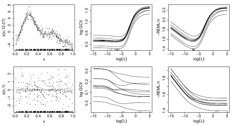
As Wood (2011) is behind a paywall, I include a copy of a similar image (the AICc results are not shown here) taken from a set of Simon's slides, available on his website, on smoothness selection methods {PDF}. The figure, from slide 10, is shown below

The two rows reflect simulated data where there is a strong (upper) or no (lower) signal respectively. The left-most panels show a realisation from each model. The remaining panels show how the GCV (middle column) and REML criteria vary as a function of $\lambda$ for 10 data sets each simulated from the real model. In the case of the upper row, notice how flat GCV is to the left of the optimum. The rug plots in these panels shows the optimal $\lambda$ for each of the 10 realisations. The REML criterion has a much more pronounced optimum and less variance in the chosen values of $\lambda$.

Hence I would suggest the approach advocated by Simon Wood for his mgcv package, namely to chose as the basis dimension something that is sufficiently large as to include the flexibility anticipated in the relationship between $y = f(x) + \varepsilon$, but not so large. Then fit the model using REML smoothness selection. If the chosen model degrees of freedom is close to the dimension specified initially, increase the basis dimension and refit.

As both @M.Berk and @BrendenDufault mention, a degree of subjectivity may be required when setting up the spline basis, in terms of selecting an appropriate basis dimension from which to fit the GAM. But REML smoothness selection has proven reasonably robust in my experience in a range of GAM applications using Wood's methods.

Wood, S.N. (2011) Fast stable restricted maximum likelihood and marginal likelihood estimation of semiparametric generalize linear models. J. Royal Statistical Society B 73(Part 1), 3--6.

Answer 2

I think your best bet lies outside the smoothing algorithms; consider model parsimony.

You allude to this, but I believe it must become your chief selection criteria. Ask yourself how many "bends" seem reasonable based on the etiology/causality of the processes being modeled. Graph the fitted splines with the plots=components(clm) statement and visually assess the fit. Perhaps the high DF splines are telling a similar story as the low DF splines, except more noisily. In that case, choose a low DF fit.

After all, GAM models are intended to be exploratory.

Having used the gcv option myself, I wonder about its performance under Poisson conditions, sparse data, etc. Maybe a simulation study is due here.

Answer 3

I typed up the following answer and then realized I have no idea if it's applicable to Poisson regression which I have no experience with. Perhaps people can answer that with some comments.

---

Personally, I like the advice of B. W. Silverman (1985) "Some aspects of the spline smoothing approach to non-parametric regression curve fitting (with discussion)." (Available without subscription here): try a range of smoothing parameters and pick the one which is most visually appealing.

As he also rightly points out in the same paper, while a subjective approach may be preferred, there is still the need for automatic methods. However, GCV is generally a poor choice as it has a tendency to undersmooth. See, for example Hurvich et al (1998) "Smoothing Parameter Selection in Nonparametric Regression Using an Improved Akaike Information Criterion" (Available without subscription here). In the same paper they propose a new criteria that may alleviate your problem, the corrected AIC which includes a small sample size correction. You may find the Wikipedia description of AICc easier to follow than the paper. The Wikipedia article also includes some good advice from Burnham & Anderson (i.e. use AICc rather than AIC regardless of sample size).

In summary, my suggestions would be, in order of preference:

1. Pick the smoothing parameter manually via visual assessment
2. Use the corrected AIC (AICc) rather than GCV
3. Use the standard AIC