1
$\begingroup$

I was wondering if I am understanding the following two points correctly:

FIRST, I think a Likelihood function for $\mu$ of a normal with a known $\sigma$ can be turned into the sampling distribution of $\bar{x}$ (sample mean), only using a scaling factor (a multiplicative constant applied to likelihood function):

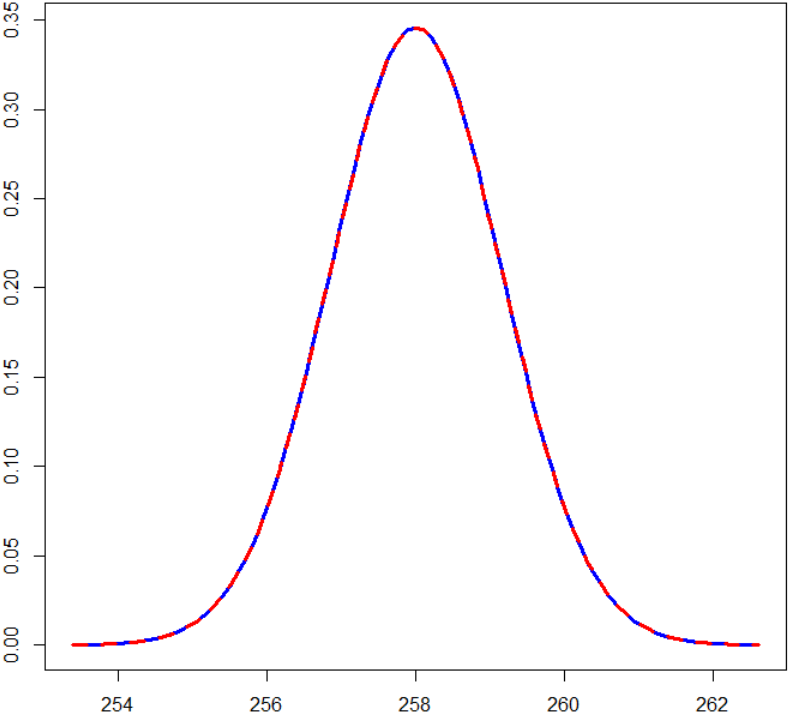
For example, in the below picture, Likelihood function for $\mu$ (solid blue) from 3 data points is multiplied by "67219744" and it matches the sampling distribution of $\bar{x}$ (dashed red), is this "process" correct for all kinds of MOTHER density functions or only for the NORMAL?

SECOND, if FIRST is always correct, can we say that whenever sampling dist. is SKEWED, Likelihood Function is also SKEWED in exactly the same way?

(please see my entire R code below the picture)

enter image description here

Here is My R code:

SIGMA = 2                  # Population SIGMA known
observations = c(250, 265, 259)  # observations drawn
n = length(observations)   # number of observations
x_bar = mean(observations) # mean of observations
SE = SIGMA / sqrt(n)       # 'S'tandard 'E'rror of the mean
x.min = x_bar - 4*SE
x.max = x_bar + 4*SE

Likelihood = function(x) sapply(lapply(x, dnorm, x = observations, SIGMA), prod)


## Sampling distribution of x_bar:
cc1 = curve(dnorm(x, x_bar, SE), from = x.min, to = x.max, col = 'blue', lwd = 3)

## Likelihood function of MU:
cc2 = curve(Likelihood, from = x.min, to = x.max, col = 'red', lwd = 3)

library(scales) ## library please install it if necessary
scale_factor = mean(rescale(cc2$y, range(cc1$y)) / cc2$y)

plot(cc1, type = "l", col = 'blue', lwd = 3) ## Sampling Dist.
lines(cc2$x, cc2$y * scale_factor, col = "red", lwd = 3, lty = 2) ## Re-sacled Likelihood
$\endgroup$
2
  • $\begingroup$ The likelihood function is usually defined as "the likelihood of a parameter value(s) given a set of data". What set of data was used to derive this likelihood function? $\endgroup$ Commented Apr 30, 2017 at 21:48
  • $\begingroup$ A likelihood function can be fairly arbitrary, but maximum likelihood estimates are commonly asymptotically normal. $\endgroup$
    – GeoMatt22
    Commented Apr 30, 2017 at 22:32

1 Answer 1

1
$\begingroup$

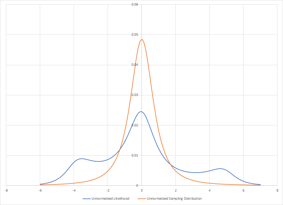
No. Consider the unnormalized likelihood and sampling distribution for the sample $\{-4,0,5\}$ drawn from $$\frac{1}{\pi}\frac{1}{1+(x-\mu)^2}.$$

enter image description here

The sampling distribution assumes infinite repetition and does not depend upon anything other than sample median. This distribution has no population mean. The likelihood depends only on the actual sample and sample statistics do not impact it at all.

While I used this because wide samples are common with this distribution, this is true for any distribution. It is just easier to make a graph with this one that shows it is not true. There is not a one to one correspondence between the sampling distribution of a parameter and the likelihood of that parameter.

$\endgroup$
11
  • $\begingroup$ @parvinkarimi under certain circumstances the sampling distribution and the posterior density will match. A normal distribution with known variance and a flat prior is one such example. An elementary example where they will not is the sampling distribution of the difference of two means $\mu_1-\mu_2$. The sampling distribution will be a t-distribution if the sample variance has been properly transformed. It will be the Behrens distribution if the variances have been marginalized out. $\endgroup$ Commented May 1, 2017 at 0:05
  • $\begingroup$ @Thanks Dave, so, if likelihood function and the sampling distribution only "under certain circumstances" match, then why "always" when put a flat prior on a parameter, the percentile-based 95% CI from a likelihood function (Bayesian Approach with flat prior) EXACTLY matches the the 95% CI from a sampling distribution (Frequentist approach)? $\endgroup$
    – rnorouzian
    Commented May 1, 2017 at 0:24
  • $\begingroup$ @parvinkarimi that certainly isn't true as there are an infinite number of $\alpha$ confidence intervals and an infinite number of $\alpha$ credible intervals. Further a flat prior, such as the uniform distribution, does not always result in the same estimator result. Consider a uniform prior with a binomial likelihood. For a sample of 5 successes out of 8 tries, the mvue/mle will be 5/8ths. The expected value for the Bayesian estimate is 3/5ths. The posterior is $504(1-\theta)^3\theta^5$. $\endgroup$ Commented May 1, 2017 at 1:00
  • $\begingroup$ @parvinkarimi any function that covers the parameter $\alpha$ percent of the time is a valid confidence interval. There are an infinite number of those functions. Likewise, any combination of segments of the parameter space that includes $\alpha$ percent of the density is a valid interval, even if unconventional. The least dense 95% percent of the parameter space and the densest 95% percent are valid credible sets. For a variety of optimality reasons, the highest density region is usually used. Also for a variety of reasons, only some confidence intervals get used. $\endgroup$ Commented May 1, 2017 at 1:13
  • $\begingroup$ @parvinkarimi in the above example, the 95% HDR for the Bayesian is (.299,.863) with a center on .6. The standard CI for the Frequentist is (.2895,.9605) with a center of .625. The Bayesian interval is more accurate than the Frequentist/Likelihoodist because it doesn't assume the point estimate is true. By making more allowance for uncertainty in the overall process, you tend to get a more precise final estimate. The Bayesian interval is 85% of the size of the Frequentist due to this difference. $\endgroup$ Commented May 1, 2017 at 1:26

Your Answer

By clicking “Post Your Answer”, you agree to our terms of service and acknowledge you have read our privacy policy.

Not the answer you're looking for? Browse other questions tagged or ask your own question.